
A SINGLE PAN AND TILT CAMERA ARCHITECTURE FOR
INDOOR POSITIONING AND TRACKING
T. Gaspar and P. Oliveira
IST/ISR, Lisboa, Portugal
Keywords:
Indoor positioning and tracking systems, Camera calibration, GVF snakes, Multiple-model adaptive estima-
tion, Single camera vision systems.
Abstract:
A new architecture for indoor positioning and tracking is proposed, based on a single low cost pan and tilt
camera, where three main modules can be identified: one related to the interface with the camera, supported
on parameter estimation techniques; other, responsible for isolating and identifying the target, based on ad-
vanced image processing techniques, and a third, that resorting to nonlinear dynamic system suboptimal state
estimation techniques, performs the tracking of the target and estimates its position, and linear and angular
velocities. To assess the performance of the proposed methods and this new architecture, a software package
was developed. An accuracy of 20cm was obtained in a series of indoor experimental tests, for a range of
operation of up to ten meter, under realistic real time conditions.
1 INTRODUCTION
With the development and the widespread use of
robotic systems, localization and tracking have be-
come fundamental issues that must be addressed in
order to provide autonomous capabilities to a robot.
The availability of reliable estimates is essential to
its navigation and control systems, which justifies the
significant effort that has been put into this domain,
see (Kolodziej and Hjelm, 2006), (Bar-Shalom et al.,
2001) and (Borenstein et al., 1996).
In outdoor applications, the NAVSTAR Global
Positioning System (GPS) has been widely explored
with satisfactory results for most of the actual needs.
Indoor positioning systems based on this technology
however face some undesirable effects, like multipath
and strong attenuation of the electromagnetic waves,
precluding their use.
Alternative techniques, such as infrared radiation,
ultrasounds, radio frequency, vision has been success-
fully exploited as reported in detail in (Kolodziej and
Hjelm, 2006), and summarized in (Gaspar, 2008).
The indoor tracking system proposed in this
project uses vision technology, since this technique
has a growing domain of applicability and allows to
achieve acceptable results with very low investment.
This system estimates in real time the position, ve-
locity, and acceleration of a target that evolves in an
unknown trajectory, in the 3D world, as well as its an-
gular velocity. In order to accomplish this purpose, a
new positioning and tracking architecture is detailed,
based on suboptimal stochastic multiple-model adap-
tive estimation techniques.
The complete process of synthesis, analysis, im-
plementation, and validation in real time exceeds the
objectives of this paper, due to space limitations. The
reader interested can found these issues discussed in
detail in (Gaspar, 2008).
This document is organized as follows. In sec-
tion 2 the architecture of the developed positioning
and tracking system is introduced, as well as the main
methodologies and algorithms developed. In section
3 the camera and lens models are briefly introduced.
To isolate and identify the target, advanced image pro-
cessing algorithms are discussed in section 4, and in
section 5, the used multiple-model nonlinear estima-
tion technique is introduced. In the last two sections,
6 and 7, experimental results of the developed sys-
tem, and concluding remarks and comments on future
work, respectively, are presented.
2 SYSTEM ARCHITECTURE
In this project a new architecture for indoor position-
ing and tracking is proposed, based on three main
523
Gaspar T. and Oliveira P. (2009).
A SINGLE PAN AND TILT CAMERA ARCHITECTURE FOR INDOOR POSITIONING AND TRACKING.
In Proceedings of the Fourth International Conference on Computer Vision Theory and Applications, pages 523-530
DOI: 10.5220/0001803105230530
Copyright
c
SciTePress
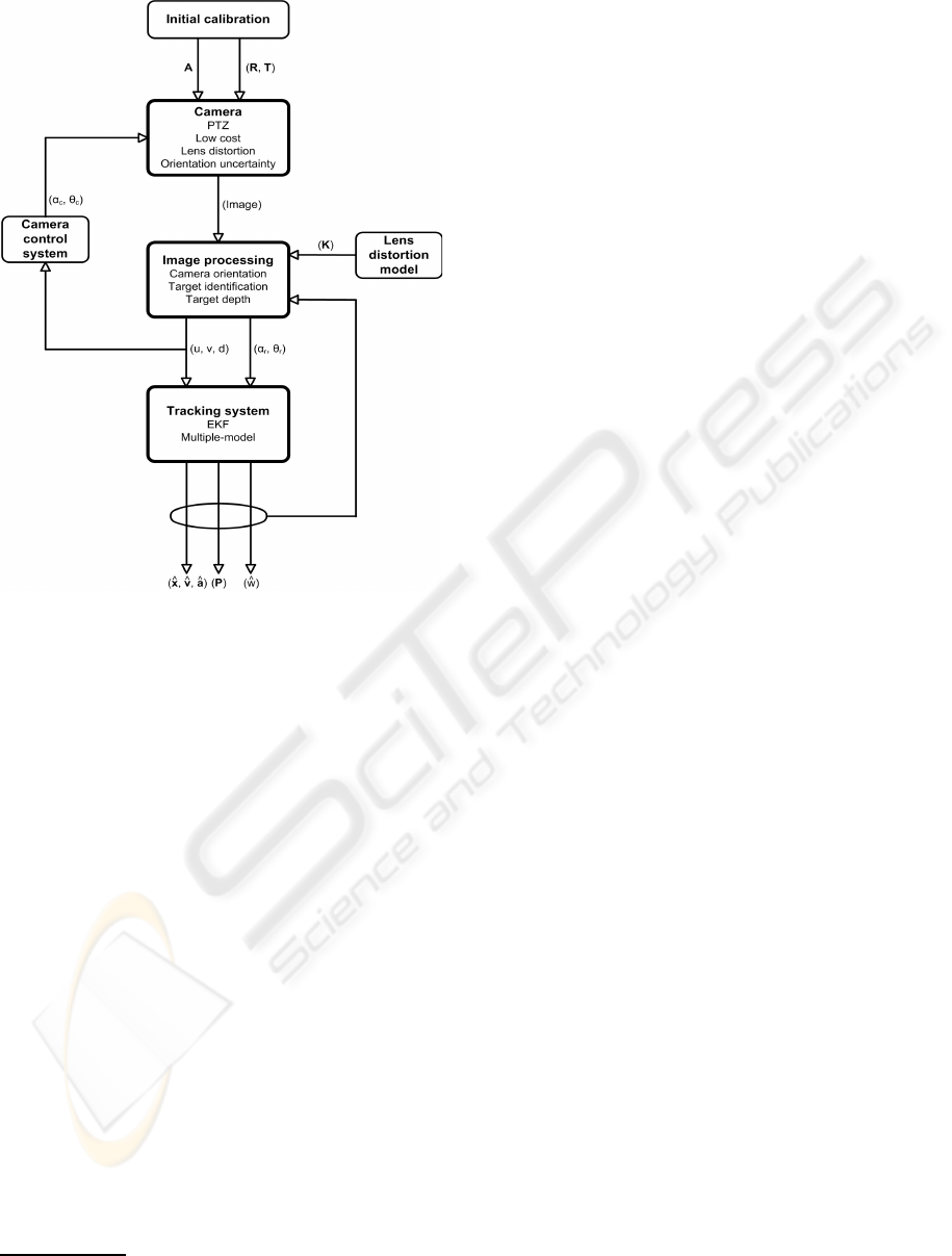
Figure 1: Tracking system architecture.
modules: one that addresses the interface with the
camera, the second that implements the image pro-
cessing algorithms, and a third responsible for dy-
namic systems state estimation. The proposed archi-
tecture is presented in Fig. 1, and is described next
1
.
The extraction of physical information from an
image acquired by a camera, requires the knowledge
of its intrinsic (A) and extrinsic (R and T) parame-
ters, which are computed during the initial calibration
process. In this paper, calibration was preceded by
an independent determination of a set of parameters
(K) responsible for compensating the distortion intro-
duced by the lens of the camera. Since the low cost
camera used has no orientation sensor, the knowledge
of its position in each moment requires the develop-
ment of an external algorithm capable of estimate its
instantaneous pan α
r
and tilt θ
r
angles.
The target identification is the main purpose of the
image processing block. An active contour method,
usually denominated as snakes, was selected to track
the important features in the image. The approach se-
lected consists of estimating the target contour, pro-
viding the necessary information to compute its cen-
1
In this section some quantities are presented informally
to augment the legibility of the whole document.
ter coordinates (u,v) and its distance (d) to the origin
of the world reference frame. These quantities corre-
spond to the measurements that are used to estimate
the position (
b
x), velocity (
b
v), and acceleration (
b
a) of
the body to be tracked. Note that the computation of d
requires the knowledge of the real dimensions of the
target, since the proposed system uses a single camera
instead of a stereo configuration.
To obtain estimates on the state and parame-
ters of the underlying dynamic system, an estima-
tion problem is formulated and solved. However, the
dynamic model adopted and the sensor used, have
nonlinear characteristics. Extended Kalman filters
were included in a multiple-model adaptive estima-
tion methodology, that provides estimates on the sys-
tem state (
b
x,
b
v, and
b
a), identifies the unknown target
angular velocity bw, and the estimation error covari-
ance P, as depicted in Fig. 1.
The command for the camera is the result of solv-
ing a decision problem, with the purpose of maintain-
ing the target close to the image center. Since the
range of movements available is restricted, the imple-
mented decision system is very simple and consists
in computing the pan and tilt angles (α
c
and θ
c
), that
should be sent to the camera at each moment. Large
distances between the referred centers are avoided,
thus the capability of the overall system to track the
targets is increased.
3 SENSOR: PTZ CAMERA
3.1 Camera Model
Given the high complexity of the camera optical sys-
tem, and the consequent high number of parameters
required to model the whole image acquisition pro-
cess, it is common to exploit a linear model to the
camera. In this architecture it was considered the clas-
sical pinhole model (Faugeras and Luong, 2001).
Let M = [x,y,z,t]
T
be the homogeneous coordi-
nates of a visible point, in the world reference frame,
and m = [u,v,s]
T
the corresponding homogeneousco-
ordinates of the same point in the image frame. Ac-
cording to this model, the relation between the coor-
dinates expressed in these two coordinate frames is
given by
λm = PM, (1)
where λ is a multiplicative constant, related with the
distance from the point in space to the camera, and
P the projection matrix that relates 3D world coor-
dinates and 2D image coordinates. The transforma-
tion given by this matrix can be decomposed into
VISAPP 2009 - International Conference on Computer Vision Theory and Applications
524

three others: one between world and camera coordi-
nate frames, expressed by
c
g
M
in homogeneous co-
ordinates; other responsible for projecting 3D points
into the image plane, represented by π, and a third
one that changes the origin and units of the coordinate
system used to identify each point in the acquired im-
ages, denoted as A. The product of the three previous
transformations results in the overall expression for
the matrix P, which is given by P = A.π.
c
g
M
, and es-
tablishes the relation between a point in the 3D world
and its correspondent in the acquired images.
The use of the previous model implies the deter-
mination of the intrinsic and extrinsic parameters re-
ferred before. In this work, the classical approach pro-
posed by Faugeras (Faugeras and Luong, 2001) was
selected and implemented. The disadvantages of this
method are: i) the required preparation of the scene in
which the camera is inserted, and ii) the distortion of
the lens is disregarded. However, the impact of these
requirements is moderate since the camera in this ap-
plication is supposed to be placed in a fixed location
in the world (the calibration needs to be performed
just once). A separate algorithm that compensates for
lens distortion is implemented, see section 3.3 for de-
tails. The major advantages are that only one image
is required and reliable results can be obtained.
The classical method proposed by Faugeras
consists in performing an initial estimation of the
projection matrix, that is done from a set of points
with known coordinates in world and camera ref-
erence frames. Writing (1) and reorganizing the
expression obtained to every one of the n points used
in the calibration process, and considering that the
index i identifies the coordinates of the i
th
used point,
yields, for each point,
x
i
y
i
z
i
1 0 0 0 0 −u
i
x
i
−u
i
y
i
−u
i
z
i
−u
i
0 0 0 0 x
i
y
i
z
i
1 −v
i
x
i
−v
i
y
i
−v
i
z
i
−v
i
.p = 0,
with
p =
p
11
p
12
p
13
p
14
p
21
p
22
p
23
p
24
p
31
p
32
p
33
p
34
T
,
where p
jk
is the P element whose line and column are
j and k, respectively.
The previous equations, when applied to the
entire set of used points, lead to a system of the
form Lp = 0, where L is a 2n × 12 matrix. The
solution of this system corresponds to the eigenvector
associated with the smallest eigenvalue of L
T
L, or,
equivalently, to the singular vector of L associated
with the smallest singular value of its Single Value
Decomposition. Since the projection matrix has 12
elements, and each point considered contributes with
two equations, there is a minimum of 6 points that
must be used in the calibration process. The intrinsic
and extrinsic parameters of the camera can then be
computed from the estimated p vector as
u
0
= p
1
.p
3
, v
0
= p
2
.p
3
,
|α
u
| = ||p
1
− u
0
p
3
||, |α
v
| = ||p
2
− v
0
p
3
||,
r
3
= p
3
, r
2
=
p
2
−v
0
r
3
α
v
,
r
1
=
p
3
−u
0
r
3
α
u
, t
z
= p
34
,
t
x
=
p
14
−u
0
t
z
α
u
, t
y
=
p
24
−v
0
t
z
α
v
,
where p
k
=
p
k1
p
k2
p
k3
, and p
i
.p
j
represents
the internal product of the vectors p
i
and p
j
, see
(Faugeras and Luong, 2001) and (Gaspar, 2008) for
details.
3.2 PTZ Camera Internal Geometry
The camera used in this project has the ability to de-
scribe pan and tilt movements, which makes possi-
ble the variation over time of its extrinsic parame-
ters. Thus, the rigorous definition of the rigid body
transformation between camera and world reference
frames implies the adoption of a model to the camera
internal geometry and the study of its direct kinemat-
ics.
Since the used Creative WebCam Live! Motion
camera has a closed architecture, its internal geome-
try model was estimated from the analysis of its ex-
ternal structure and based on a small number of ex-
periments.
The proposed model considers five transforma-
tions, that include the pan, tilt, and roll angles be-
tween the world and camera reference frames; the off-
set between the origin of the world reference frame
and the camera rotation center, and the offset between
the camera rotation and optical centers.
The composition of this transformations leads to
the global transformation between world and camera
reference frames:
c
g
M
=
M
g
−1
c
,
M
g
c
=
M
g
0
0
g
1
1
g
2
2
g
3
3
g
c
,
that is fundamental to determine the camera projec-
tion matrix over time.
The expressions introduced require, however, the
knowledge of five parameters: pan, tilt and roll an-
gles, the position of the camera optical center in the
world coordinate frame, when these angles are zero,
and the offset between this point and the camera ro-
tation center. Since there is no position sensor in
the camera, its orientation must be determined in real
time using reference points in the 3D world. The po-
sition of the camera optical and rotation centers, when
the pan and tilt angles are zero, can be performed on
an initial stage resorting to points of the world with
known coordinates.
A SINGLE PAN AND TILT CAMERA ARCHITECTURE FOR INDOOR POSITIONING AND TRACKING
525

3.3 Lens Distortion
The mapping function of the pinhole camera between
the 3D world and the 2D camera image is linear, when
expressed in homogeneous coordinates. However, if a
low-cost or wide-angle lens system is used, the linear
pinhole camera model fails. In those cases, and for the
camera used in this work, the radial lens distortion is
the main source of errors and no vestige of tangential
distortion was identified. Therefore, it is necessary to
compensate this distortion by a nonlinear inverse ra-
dial distortion function, which corrects measurements
in the 2D camera image to those that would have been
obtained with an ideal linear pinhole camera model.
The inverse radial distortion function is a map-
ping that recoversthe coordinates (x, y) of undistorted
points from the coordinates (x
d
,y
d
) of the correspon-
dent distorted points, where both coordinates are re-
lated to a reference frame with origin in image dis-
tortion center (x
0
,y
0
). Since radial deformation in-
creases with the distance to the distortion center, the
inverse radial distortion function f(r
d
) can be ap-
proximated and parameterized by a Taylor expansion
(Thormahlen et al., 2003), that results in
x = x
d
+ x
d
∞
∑
i=0
k
i
r
i−1
d
and y = y
d
+ y
d
∞
∑
i=0
k
i
r
i−1
d
,
where
r
d
=
q
x
2
d
+ y
2
d
.
The lens distortion compensation method adopted
in this project is independent of the calibration pro-
cess responsible for determining the pinhole model
parameters, and is based on the rationale that straight
lines in the 3D space must remain straight lines in 2D
camera images. Ideally, if acquired images were not
affected by distortion, 3D world straight lines would
be preserved in 2D images. Hence, the inverse radial
distortion model parameters estimation was based on
the resolution of the following set of equations
f
i1
= (y
i1
− by
i1
(m
i
,b
i
,x
i1
))
2
= 0
.
.
.
f
iN
p
= (y
iN
p
− by
iN
p
(m
i
,b
i
,x
iN
p
))
2
= 0
i = 1,..., N
r
with
by
ij
(m
i
,b
i
,x
ij
) = m
i
x
ij
+ b
i
,
where N
r
and N
p
are the number of straight lines and
points per straight line acquired from the distorted im-
age, respectively. A set of N
r
∗N
p
nonlinear equations
results, its solution can be found resorting to the New-
ton’s method, and estimates for the parameters k
3
, k
5
,
x
0
, y
0
, m
i
, b
i
, i = 1,... , N
r
are obtained. vfill
4 IMAGE PROCESSING
4.1 Target Isolation and Identification
The isolation and identification of the target to be
tracked in each acquired image is proposed to be tack-
led resorting to an active contours method. Active
contours (Kass et al., 1987), or snakes, are curves de-
fined within an image domain that can move under the
influence of internal forces coming from within the
curve itself and external forces computed from the im-
age data. The internal and external forces are defined
so that the snake will conform to an object boundary
or other desired features within an image. Snakes are
widely used in several computer vision domains, such
as edge detection (Kass et al., 1987), image segmen-
tation (Leymarie and Levine, 1993), shape modeling
(Terzopoulos and Fleischer, 1988), (McInerney and
Terzopoulos, 1995), or motion tracking (Leymarie
and Levine, 1993), as happens in this application.
In this project a parametric active contour method
is used (Kass et al., 1987), in which a parameterized
curve x(s) = [x(s),y(s)], s ∈ [0,1], evolves over time
towards the desired image features, usually edges, at-
tracted by external forces given by the negative gra-
dient of a potential function. The evolution occurs in
order to minimize the energy of the snake
E
sk
= E
int
+ E
ext
,
that, as can be seen, includes a term related to its inter-
nal energy E
int
, which has to do with its smoothness,
and a term of external energy E
ext
, based on forces ex-
tracted from the image. Traditionally, this energy can
be expressed in the form
E
sk
=
Z
1
0
1
2
[α|x
′
(s)|
2
+ β|x
′′
(s)|
2
] + E
ext
(x(s))ds,
(2)
where the parameters α and β control the snake ten-
sion and rigidity, respectively, and x
′
(s) and x
′′
(s) de-
note the first and second derivatives of x(s) with re-
spect to s.
Approximating the solution of the variational for-
mulation (2) by the spacial finite differences method,
with step h, yields
(x
t
)
i
=
α
h
2
(x
i+1
− 2x
i
+ x
i−1
) −
β
h
4
(x
i+2
− 4x
i+1
+
+ 6x
i
− 4x
i−1
+ x
i−2
) + F
(p)
ext
(x
i
),
where x
i
= x(ih,t), and F
(p)
ext
(x
i
) represents the image
influence at the point x
i
.
The temporal evolution of the active contour in the
image domain occurs according to the expression
x
n+1
= x
n
+ τx
n
t
,
VISAPP 2009 - International Conference on Computer Vision Theory and Applications
526

where τ is the considered temporal step. The iterative
process ends when the coordinates of each point of
the snake remain approximately constant over time.
4.2 Sensor Measurements
Once obtained the target contour, it is possible to
compute the measurements that will be provided to
the estimation process: the target center coordinates
(u,v), and its distance (d) to the origin of world refer-
ence frame.
Target center coordinates in each acquired image
are computed easily as being the mean of the coordi-
nates of the points that belong to the target contour.
Target distance to the origin of world reference frame
is computed from its estimated boundary. Its real di-
mensions in the 3D world, and the knowledge of the
camera intrinsic and extrinsic parameters, allows to
establish metric relations between image and world
quantities. Estimates on the depth of the target can
then be obtained. A complete stochastic characteriza-
tion can be found in (Gaspar, 2008) and will be the
measurements considered as inputs to the estimation
method used.
The use of triangulation methods for at least two
cameras, would allow the computation of the tar-
get distance without further knowledge on the target.
However, the present tracking system uses a single
camera. Thus, additional information must be avail-
able. In this work, it is assumed that the target dimen-
sions are known.
5 TRACKING SYSTEM
In this section, the implemented nonlinear estimation
methods is described. Estimates on the target posi-
tion, velocity and acceleration, in the 3D world, are
provided and angular velocity is identified. This esti-
mator is based on measurements from the previously
computed target center coordinates and distance to the
origin of world reference frame.
5.1 Extended Kalman Kilter
The Kalman filter (Gelb, 2001) provides an optimal
solution to the problem of estimating the state of
a discrete time process that is described by a lin-
ear stochastic difference equation. However, this ap-
proach is nod valid when the process and/or the mea-
surements are nonlinear. One of the most successful
approaches, in these situations, consists in applying
a linear time-varying Kalman filter to a system that
results from the linearization of the original nonlin-
ear one, along the estimates. This kind of filters are
usually referred to as Extended Kalman filters (EKF)
(Gelb, 2001), and have the advantage of being com-
putationally efficient, which is essential in real time
applications.
Consider a nonlinear system with state x ∈ ℜ
n
ex-
pressed by the nonlinear stochastic difference equa-
tion
x
k
= f(x
k−1
,u
k−1
,w
k−1
),
and with measurements available z ∈ ℜ
m
given by
z
k
= h(x
k
,v
k
),
where the index k represents time, u
k
the control
input, and w
k
∈ ℜ
n
and v
k
∈ ℜ
m
are random vari-
ables that correspond to the process and measurement
noise, respectively. These variables are assumed to
be independent, i.e. E[w
k
v
k
T
] = 0, and with Gaus-
sian probability density functions with zero mean and
covariance matrices Q
k
and R
k
, respectively.
In the case of linear dynamic systems, the esti-
mates provided by the Kalman filter are optimal, in
the sense that the mean square estimation error is min-
imized. Estimates computed by EKF are suboptimal.
It is even possible that it does not converge to the sys-
tem state in some situations. However, the good per-
formance observed in many practical applications, re-
vealed this strategy as the most successful and popular
in nonlinear estimation.
The implementation of an EKF requires a math-
ematical model to the target and sensors used. The
choice of appropriate models is extremely important
since it improves significantly the target tracking sys-
tem performance, reducing the effects of the limited
observation data available in this kind of applications.
Given the movements expected for the targets to be
tracked, the 3D Planar Constant-Turn Model as pre-
sented in (Li and Jilkov, 2003), was selected. This
model considers the vector x = [x,
˙
x,
¨
x,y,
˙
y,
¨
y,z,
˙
z,
¨
z]
T
as the state of the target, where [x,y,z], [
˙
x,
˙
y,
˙
z], and
[
¨
x,
¨
y,
¨
z] are the target position, velocity, and accelera-
tion in the world, respectively.
The sensor measurements available in each time
instant correspond to the target center coordinates
(u,v) and target distance (d) to the origin of world
reference frame, and are given by
u =
p
11
x+ p
12
y+ p
13
z+ p
14
p
31
x+ p
32
y+ p
33
z+ p
34
+ v
u
v =
p
21
x+ p
22
y+ p
23
z+ p
24
p
31
x+ p
32
y+ p
33
z+ p
34
+ v
v
d =
p
x
2
+ y
2
+ z
2
+ v
d
,
where p
ij
is the projection matrix element in the line i
and column j, and v = [v
u
,v
v
,v
d
]
T
is the measurement
A SINGLE PAN AND TILT CAMERA ARCHITECTURE FOR INDOOR POSITIONING AND TRACKING
527

noise (the time step subscript k was omitted for sim-
plicity of notation). The measurement vector is given
by z = [u,v,d]
T
.
Next, a standard notation is used (see (Gelb, 2001)
for details) to describe each Kalman filter:
Predict step
b
x
−
k
= f(
b
x
k−1
,u
k−1
,0)
P
−
k
= A
k
P
k−1
A
T
k
+ W
k
Q
k−1
W
T
k
Update step
K
k
= P
−
k
H
T
k
(H
k
P
−
k
H
T
k
+ V
k
R
k
V
T
k
)
−1
b
x
k
=
b
x
−
k
+ K
k
(z
k
− h(
b
x
−
k
,0))
P
k
= (I− K
k
H
k
)P
−
k
,
where K
k
is the Kalman filter gain.
The complete measurement process characteriza-
tion requires also the definition of the measurement
noise covariance matrix R. This matrix can be ob-
tained from an accurate study of the available sensors,
which, in this project, consisted in executing a set of
experiments aiming to compute the standard devia-
tion of the estimation error in the image coordinates
of a 3D world point, and the standard deviation of the
error in target depth estimation.
5.2 Multiple-model
The model considered for the target requires the
knowledge of its angular velocity. However, this
value is not known in real applications, which led
us to the application of a multiple model based ap-
proach, identifying simultaneously some parameters
of the system and estimating its state.
The implemented method, known as Multiple-
Model Adaptive Estimation (MMAE) (Athans and
Chang, 1976), considers several models to a system
that differ in a parameter set (in this case the target
angular velocity). Each one of these models includes
an extended Kalman filter, whose state estimates are
mixed properly. The individual estimates are com-
bined using a weighted sum with the a posteriori hy-
pothesis probabilities of each model as weighting fac-
tors, leading to the state estimate
b
x
k
=
N
∑
j=1
p
j
k
b
x
j
k
,
with covariance matrix
P
k
=
N
∑
j=1
p
j
k
[P
j
k
+ (
b
x
j
k
−
b
x
k
)(
b
x
j
k
−
b
x
k
)
T
],
where p
j
k
corresponds to the a posteriori probability
of the model j, at the time instante k, and N to the
number of considered models.
It should be stressed that the methods used to com-
pute the a posteriori probabilities of each model and
the final state estimate are optimal if each one of the
individual estimates is optimal. However, this is not
the case in this application, since the known solu-
tions to nonlinear estimation problems at present do
not provide optimal results.
6 EXPERIMENTAL RESULTS
In this section some brief considerations about the
developed positioning and tracking system are ad-
vanced, and the experimental results of its application
to real time situations are presented.
6.1 Application Description
The architecture for positioning and tracking pro-
posed in this project was implemented in Matlab, and
can be divided into three main modules: one that ad-
dresses the interface with the camera, other that im-
plements the image processing algorithms, and a third
related to the estimation process.
Interface with the Camera. Since the camera used
in this project has a discrete and limited range of
movements, its orientation in each time instant is de-
termined according to a decision system whose aim is
to avoid that the distance between the image and the
target centers exceed certain values.
The CCD sensor built-in the camera acquires im-
ages with a maximum dimension of 640× 480 pixels,
which is the resolution chosen for this applica-
tion. Despite its higher computational requirements,
smaller targets can be tracked with an increase on the
accuracy of the system.
Image Processing. The active contour method was
implemented with the values of α and β equal to 0.5
and 0.05, respectively, since these values were the
ones that led to better results.
The developed application is optimized to follow
red targets, whose identification in acquired images is
easy, since image segmentation is itself a very com-
plex domain, and does not correspond to the main fo-
cus of this work.
Estimation Process. The adopted MMAE approach
was based on the utilization of four initially equiprob-
able target models, that differ on target angular veloc-
ity values: 2π
1
50
[0,1,2,3]rad/s.
Each one of the models requires the knowledge
of the power spectral density matrix of the process
noise, that is not available. After some preliminary
tuning, the matrix considered for this quantity was
set to diag[0.1,0.1,0.1].
VISAPP 2009 - International Conference on Computer Vision Theory and Applications
528
The sampling interval of the developed applica-
tion was made variable, however for the parameters
previously discussed, a lower bound of approximately
0.5s was found.
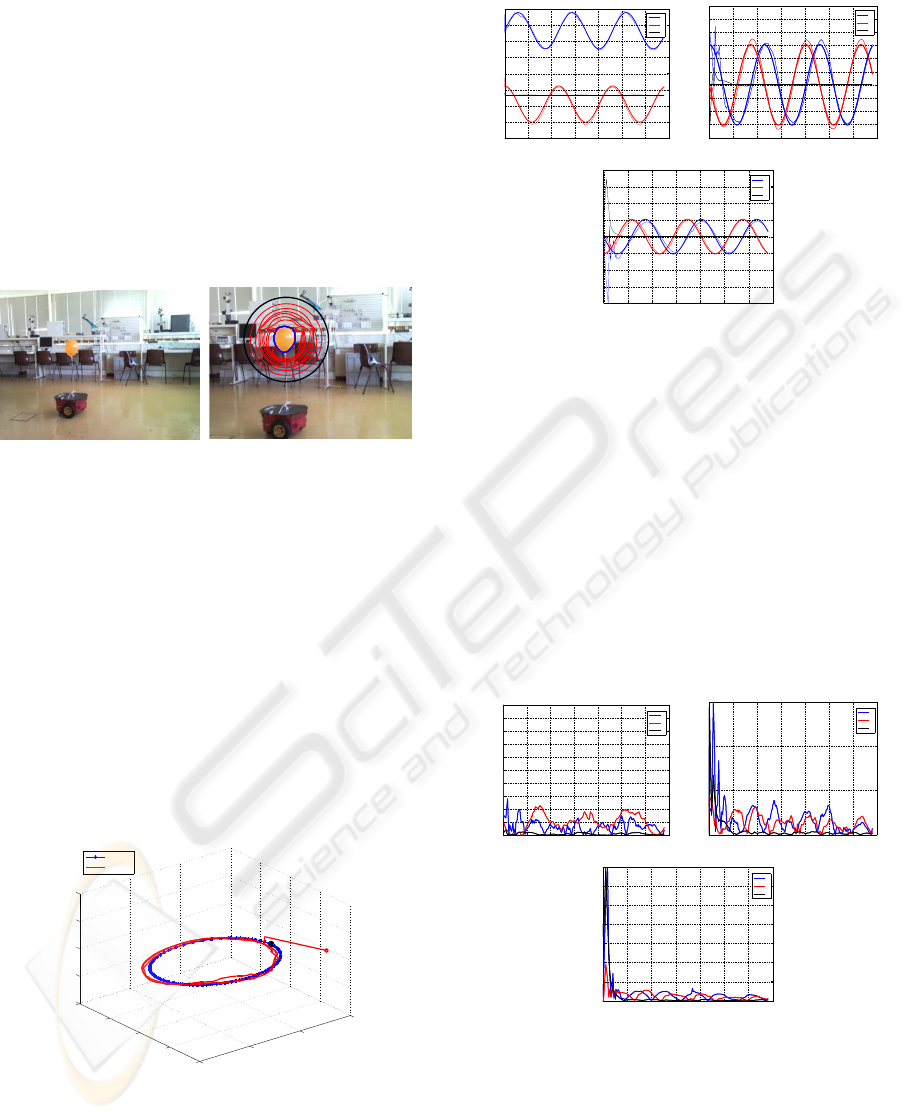
6.2 Application Performance
The results presented in this section are relative to the
tracking of a red balloon attached to a robot Pioneer
P3-DX, as depicted in Fig. 2, programmedto describe
a circular trajectory.
Figure 2: Real time target tracking. Left: Experimental
setup; Right: Target identification, where the initial snake
is presented in black, its temporal evolution is presented in
red, and the contour final estimate is presented in blue.
In Fig. 3, the 3D nominal and estimated target tra-
jectories are presented. The target position, velocity
and acceleration along time are depicted in Fig. 4.
Despite the significant initial uncertainty in the state
estimate, the target position, velocity, and accelera-
tion estimates converge to the vicinity of the real val-
ues. Moreover, given the suboptimal nature of the re-
sults produced by the extended Kalman filter in non-
linear applications, in some experimental cases where
an excessively poor initial state estimate was tested,
divergence of the filter occurred.
1000
2000
3000
4000
5000
−2000
−1000
0
1000
−1500
−1000
−500
0
500
Y
X
Z
Real
MMAE
Figure 3: 3D position estimate of a real target. The real
position of the target in the initial instant is presented in
black.
The position, velocity, and acceleration estima-
tion errors are presented in Fig. 5. These quantities
0 20 40 60 80 100 120 140
−3000
−2000
−1000
0
1000
2000
3000
4000
5000
M
X [mm]
t [s]
x
y
z
0 20 40 60 80 100 120 140
−200
−150
−100
−50
0
50
100
150
200
250
300
v [mm/s]
t [s]
x
y
z
0 20 40 60 80 100 120 140
−80
−60
−40
−20
0
20
40
60
80
a [mm/s
2
]
t [s]
x
y
z
Figure 4: Position (top left pan), velocity (top right pan),
and acceleration (bottom pan) estimates of a real target in
the world. The slender and tickler lines correspond to the
estimated and real values, respectively.
have large transients in the beginning of the experi-
ment, due to the initial state estimation error, and de-
crease quickly to values beneath 20cm, 4cm/s, and
0.5cm/s
2
, respectively. There are several reasons that
can justify the errors observed: i) the uncertainty as-
sociated with the characterization of the real trajec-
tory described by the target, and ii) possible mis-
matches between the models considered for the cam-
era and target, and iii) incorrect measurement and sen-
sor noise characterization.
0 20 40 60 80 100 120 140
0
100
200
300
400
500
600
700
800
900
1000
|e
p
| [mm]
t [s]
x
y
z
0 20 40 60 80 100 120 140
0
50
100
150
|e
v
| [mm/s]
t [s]
x
y
z
0 20 40 60 80 100 120 140
0
10
20
30
40
50
60
70
|e
a
| [mm/s
2
]
t [s]
x
y
z
Figure 5: Position (top left pan), velocity (top right pan),
and acceleration (bottom pan) estimation error of a real tar-
get in the world.
The results of the adopted MMAE approach are
presented in Fig. 6. For the trajectory reported, the
real target angular velocity is 2π0.0217rad/s. Thus,
the probability associated to the model closer to the
real target tends to 1 along the experiment, as depicted
A SINGLE PAN AND TILT CAMERA ARCHITECTURE FOR INDOOR POSITIONING AND TRACKING
529

on the left panel of Fig. 6. On the right panel of that
figure, the real and estimated angular velocities are
plotted.
0 20 40 60 80 100 120 140
0
0.1
0.2
0.3
0.4
0.5
0.6
0.7
0.8
0.9
1
probabilidades
t [s]
p1
p2
p3
p4
0 20 40 60 80 100 120 140
0
0.01
0.02
0.03
0.04
0.05
0.06
w [º/s]
t [s]
w estimado
w real
4 modelos
Figure 6: MMAE evolution over time. On the left, the a
posteriori hypothesis probabilities. On the right, real (red)
and estimated (blue) target angular velocity.
In what concerns the range of operation for the
proposed system, it depends significantly on the cam-
era used and on the size of the target to be tracked. In
the experiments reported, an elliptic shape with axes
of length 106mm and 145mm, was identified and lo-
cated, with the mentioned accuracies for distances up
to approximately 7m from the camera. The lower
bound of the range of distances in which the appli-
cation works properly, is limited by the distance at
which the target stops being completely visible, filling
the camera field of vision. For the target considered,
this occurs at distances bellow 40cm.
7 CONCLUSIONS AND FUTURE
WORK
A new architecture for indoor positioning and track-
ing is presented, supported on suboptimal stochastic
multiple-model adaptive estimation techniques. The
proposed approach was implemented using a single
low cost pan and tilt camera, estimating the real time
location of a target which moves in the 3D real world
with accuracies on the order of 20cm.
The main limitations of the implemented system
are the required knowledge on the target dimensions,
and the inability to identify targets with colors other
than red.
In the near future, an implementation of the de-
veloped architecture in C will be pursued, which will
allow for the tracking of more unpredictable targets.
Also, an extension of the proposed architecture to a
multiple camera based system is thought. Distances
to targets will then be computed resorting to triangu-
lation methods, thus avoiding the requirement on the
precise knowledge of their dimensions.
Finally, it is also advised the integration of a sen-
sor in the vision system that retrieves camera orienta-
tion in each time instant, and the implementation of
an image segmentation algorithm that can identify a
wider variety of targets.
ACKNOWLEDGEMENTS
This work was partially supported by Fundac¸˜ao
para a Ciˆencia e a Tecnologia (ISR/IST plurian-
ual funding) through the POS Conhecimento Pro-
gram that includes FEDER funds and by the project
PDCT/MAR/55609/2004 - RUMOS of the FCT.
REFERENCES
Athans, M. and Chang, C. (1976). Adaptive Estimation
and Parameter Identification using Multiple Model
Estimation Algorithm. MIT Lincoln Lab., Lexington,
Mass.
Bar-Shalom, Y., Rong-Li, X., and Kirubarajan, T. (2001).
Estimation with Applications to Tracking and Naviga-
tion: Theory Algorithms and Software. John Wiley &
Sons, Inc.
Borenstein, J., Everett, H. R., and Feng, L. (1996). Where
am I? Sensors and Methods for Mobile Robot Posi-
tioning. Editado e compilado por J. Borenstein.
Faugeras, O. and Luong, Q. (2001). The geometry of multi-
ples images. MIT Press.
Gaspar, T. (2008). Sistemas de seguimento para aplicac¸˜oes
no interior. Master’s thesis, Instituto Superior
T´ecnico.
Gelb, A. (2001). Applied Optimal Estimation. MIT Press,
Cambridge, Massachusetts.
Kass, M., Witkin, A., and Terzopoulos, D. (1987). Snakes:
Active contour models. Int. J. Comput. Vis., 1:321–
331.
Kolodziej, K. and Hjelm, J. (2006). Local Positioning Sys-
tems: LBS Applications and Services. CRC Press.
Leymarie, F. and Levine, M. D. (1993). Tracking de-
formable objects in the plane using an active contour
model. IEEE Trans. Pattern Anal. Machine Intell.,
15:617–634.
Li, X. R. and Jilkov, V. P. (2003). Survey of maneuvering
target tracking. part i: Dynamic models. IEEE Trans-
actions on Aerospace and Electronic Systems, pages
1333–1364.
McInerney, T. and Terzopoulos, D. (1995). A dynamic finite
element surface model for segmentation and tracking
in multidimensional medical images with application
to cardiac 4d image analysis. Comput. Med. Imag.
Graph, 9:69–83.
Terzopoulos, D. and Fleischer, K. (1988). Deformable mod-
els. Vis. Comput., 4:306–331.
Thormahlen, T., Broszio, H., and Wassermann, I. (2003).
Robust line-based calibration of lens distortion from a
single view. Mirage 2003, pages 105–112.
VISAPP 2009 - International Conference on Computer Vision Theory and Applications
530
