
A NEW APPLICATION FOR 3D-SNAKES
Modelling Electrical Discharges
Gilmario Barbosa dos Santos
University of State of Santa Catarina, UDESC-DCC, Joinville-SC, Brazil
Sidney Pinto da Cunha
Center of Information Technology Renato Archer, CTI-DRVC, Campinas-SP, Brazil
Clesio Luiz Tozzi
University of Campinas, UNICAMP-FEEC-DCA, Campinas-SP, Brazil
Keywords:
B-spline, Snakes, 3D image reconstruction, Camera calibration, Electrical discharges characterization.
Abstract:
A new approach for modelling electrical discharges is proposed. To this purpose, an active contour named 3D-
snake is used that is geometrically represented by a B-spline which evolves in 3D space constrained by internal
and external energies. More specifically, this external energy come from a pair of images. This new model is
much less dependent on determination of homologous points than the approaches found in the literature for
recovering 3D geometry of electrical discharges. In addition, the proposal discussed here is capable of tracking
the evolution os the electrical discharge taking into account the time dependence between consecutive pairs of
frames in two videos.
1 INTRODUCTION
Computer vision techniques have applied stereopsis
in images of electrical discharges. Some works as
MacAlpine and Qiu (MacAlpine et al., 1999), Qiu et
al. (Qiu and MacAlpine, 2000; Qiu et al., 1999) and
Amarasinghe et al. (Amarasinghe et al., 2007) present
some important results in this field but their strategies
are strongly dependent on explicit methods of homol-
ogous determination, and furthermore these methods
are applied for electrical discharges with low level of
curvature and wavy discharges are avoided in their ex-
periments. On the other hand, here we propose a new
approach based on 3D snakes for modelling the longi-
tudinal medial-axes of electrical discharges based on
two digital videos which practically makes correspon-
dences determination unnecessary.
In the bi-dimensional case ((Kass et al., 1988)),
the snakes are modelled by a energy funcional that
is minimized under certain constraints, as a conse-
quence the snake deforms itself looking for some fea-
ture of interest in the image. The 3D snake is a model
based on the same principles, which means that the
3D snake also has a functional of energy with geo-
metric and photometric constraints. The aspect that
differentiates 3D snake is related to its external energy
which is extracted from more than one image, which
means that the external energy must come from 2D
spaces determining a 3D force, i.e., the external en-
ergy emerges from a stereo pair of images.
Although very commonly applied in solving the
functional in bi-dimensional snakes, neither Dynamic
Programming (Amini et al., 1988) nor Greedy Algo-
rithms (Williams and Shah, 1992) are useful in the
case of 3D snakes. The approach here is based on
Ca˜nero (Canero et al., 2000; Canero, 2002) which
does not explore the methods based on meta heuris-
tic.
In the stereopsis of two digital videos, the key as-
pect in recovering a 3D global/world point from im-
ages, is the identification of homologous points in the
images. Finding homologous points is a hard problem
in stereopsis, although correlation is usually applied
for this sake but sometimes does not succeed. Consid-
546
Barbosa dos Santos G., Pinto da Cunha S. and Luiz Tozzi C. (2009).
A NEW APPLICATION FOR 3D-SNAKES - Modelling Electrical Discharges.
In Proceedings of the Fourth International Conference on Computer Vision Theory and Applications, pages 546-553
DOI: 10.5220/0001803205460553
Copyright
c
SciTePress
ering a sequence (or video) of stereo pairs of electri-
cal discharge, the 3D-snake approach practically dis-
pense the homologous determination.
The methodology for validating the approach de-
scribed here is based on a set of images built by the
simulation of an image acquisition system that cap-
tures a mathematical curve in evolution in 3D space.
After validation the method was applied on electrical
arcs stereo pairs.
In the next section (2) will be described the pre-
cursor snake model and a the 3D snake model (3).
Following a description of the experiment develpment
is given and the results reported (section 4). Finally,
the approach is applied on images of electrical dis-
charges.
2 THE PRECURSOR SNAKE
MODEL
The model of snakes was first proposed by Kass et
al. (Kass et al., 1988), it is a physical inspired model
based on the functional of energy below.
E
total
=
Z
1
0
E
int
(v(s)) + E
ext
(v(s))ds. (1)
In the Eq. (1), the snake is the contour v(s) and
coordinates x and y are determined by the parame-
ter s, so v(s) = (x(s), y(s)), and the precursor snake
can be seen as defined in a bi-dimensional cartesian
space. The external energy E
ext
(v(s)) represents the
photometric constraint originated from the image and
should be defined conveniently in order to generate
the force to guide the snake to the object of interest
in the image. In turn, the internal energy E
int
(v(s))
is the geometric constraint representing the smooth-
ness grade (first and second order of continuity) of
the active contour. This aspect can be distinguished
by checking the definition of the internal energy. Note
that, according to Eq. (2) below, the terms
∂v(s)
∂s
and
∂
2
v(s)
∂s
2
determine the first and second order continuity,
respectively. Also observe that the forces originated
by internal energy are intrinsic characteristics of the
snake.
In Eq.(2), the parameters α and β weigh the terms
in order to control the geometry of the contour defin-
ing how much of it could be wavy or not.
E
int
(v(s)) =
1
2
Z
1
0
α(s) ∗
∂v(s)
∂s
2
+ β(s) ∗
∂
2
v(s)
∂s
2
2
!
d(s). (2)
In terms of numerical methods the functional is
solved by the relaxation according to equations (3)
and (4) below (Kass et al., 1988), where α and β are
introduced in the pentadiagonal matrix A, described
in (Ihlow and Seiffert, 2005) and (Kass et al., 1988),
called stiffness matrix. The γ parameter is used for
weighing the external forces.
x
t
= (A + γI)
−1
(x
t−1
− F
x
) (3)
y
t
= (A + γI)
−1
(y
t−1
− F
y
) (4)
In fact, Eq. (3) and Eq. (4) can be compressed into
Eq. (5), where v
t
= (x
t
, y
t
) is a point of the snake in bi-
dimensional space and F corresponds to the external
force composed by F
x
, F
y
.
v
t
= (A + γI)
−1
(v
t−1
− F) (5)
Although has been initially proposed in 1988 the
active contours is still alive as can be seen in recent
works such as (Thevenaz and Unser, 2008).
3 3D-SNAKE
The 3D-snake is similar to the 2D precursory model
described above but the functional has external ener-
gies defined in 3D space and the external forces act
upon the control points of a B-spline which represents
the 3D-snake geometrically.
The 3D-snake corresponds to a B-spline which de-
forms itself in 3D space in order to match its projec-
tions with a pair of features of interest in two images.
As mentioned before, the external force is recovered
from a pair of images (in fact a pair of vectorial maps)
through triangulation, see Trucco and Verri (Trucco
and Verri, 1998) or another stereo vision method. It
is important to note that for 3D-snakes the external
force does come from the same dimensional space of
the snake itself. This aspect is an important difference
to the prior snake model proposed by Kass et al. (Kass
et al., 1988). Since, in that case the snake evolved in
the same bi-dimensional space from where the exter-
nal forces were extracted.
The 3D-snakes implemented here were inspired
mainly in the works of Ca˜nero (Canero et al., 2000;
Canero, 2002).
3.1 Initialization
Ca˜nero in (Canero et al., 2000; Canero, 2002) de-
scribes a manual determination of homologous from
which a set of 3D points are recovered for initializa-
tion of the first 3D-snake. In the proposal described
here, the initialization almost dispense homologous
determination and consists of automatic procedure.
This initialization will be described in details later
on. The next paragraphs are focused in describing the
A NEW APPLICATION FOR 3D-SNAKES - Modelling Electrical Discharges
547
steps needed to get the first 3D-snake after determina-
tion of the initial 3D points.
The inaccurate set of 3D points is approximated
(not interpolated) by a third order piecewise polino-
mial B-spline which will represent the 3D-snake. An
interpolation would force the B-spline to go through
all of the 3D data points which is not convenient be-
cause the B-spline resultant will be very wavy. So,
the best choice is doing an approximation in order
to obtain a smooth B-spline which does not neces-
sarily pass through every 3D data points; Rogers and
Adams (Rogers and Adams, 1990) provides practical
methods in order to solve this problem.
The functional of energy associated is defined
and the 3D-snake deforms by minimization of this
functional under geometrical and photometrical con-
straints. This minimization process leads the control
points of the B-spline in order to guide the projections
of the points generated by the B-spline (3D-snake) in
the direction of the features of interest in the pair of
images. When the projections match the features that
have been pointed out, the best configuration of the
3D-snake will have been reached and consequently
the best 3D spatial location of the longilineous object
represented by the snake.
For a clearer understanding, consider a pair of
videos with k pairs of frames obtained in time i ∈
0, 1, ..., k − 1. The proposal is to adjust the 3D snake
B
i
, to the pair of vectorial maps (m
1
i+1
,m
2
i+1
) repre-
senting external forces in time i + 1. So, after time
k− 1 all of the possible configuration of the 3D snake
will be covered and consequently the object repre-
sented by the 3D-snake will be tracked. Since the
cameras have been calibrated it is even possible to
measure this object.
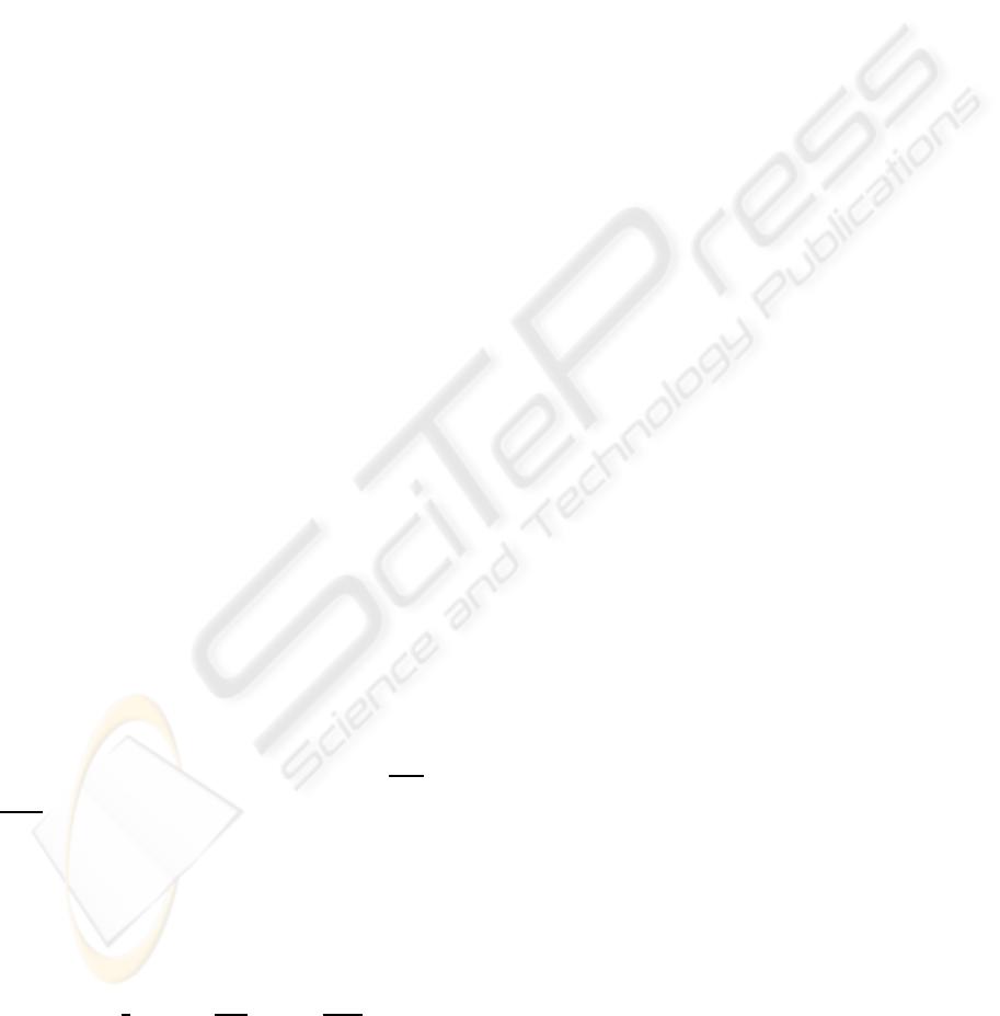
Figure 1: The external force is recovered from the space of
vectorial maps. The resultant 3D vector acts over the nodes
of the 3D-snake (in fact upon the control points of the B-
spline that represents it) deforming it in order to adapt its
own projections over a pair of images.
3.2 The Functional of Energy
The initialization gives the third order B-spline B
0
,
it is custumary to describe a B-spline by a matricial
equation like in Eq. (6), where Q represents a point
generated by the B-spline through the set of control
points V and the basis functions matrix N. This ma-
tricial formulation will be used here.
Q = NV (6)
The deformation of the 3D snake is defined by a func-
tional of energy which is very similar to the one pre-
sented in Eq. (1) but here the active contour is repre-
sented by a B-spline:
E(Q) =
Z
E
int
(Q) + E
ext
(Q)ds. (7)
Similarly to Kass et al. (Kass et al., 1988), the E
int
preserves smoothness at the same time that E
ext
is re-
sponsible for the forces which attract the 3D-snake,
pushing into the features of interest captured in the
images. Again, the minimization occurs by relaxation
such as is defined in Eq. (8), which is similar to Eq.
(5) except that here the minimization acts on the con-
trol points of the B-spline, so that a new set of control
points V
t
is calculated based on the old set V
t−1
:
V
t
= (H+ γI)
−1
(γV
t−1
− g(Q
t−1
)) (8)
Moreover, other important aspects and some sim-
ilarities between Eq. (8) and Eq. (5) must be empha-
sized, as follows:
• Note, the matrix H corresponds to the stiffness
matrix A as seen in Eq. (5). The construction
of H will be discussed later.
• The vector g(Q) corresponds to the external force
transformed into the space of control points,
therefore, the term V
t−1
− g(Q) attracts the con-
trol points and consequently Q(s) in the direction
of the features of interest depicted in the images.
For calculating g(Q) Ca˜nero (Canero, 2002) rec-
ommends the approximation described in Eq. (9),
where N is the basis functions matrix used in Eq.
(6):
g(Q) ≈ N
T
F
ext
(Q) (9)
• The external force F
ext
is recovered from vectorial
maps (from 2D to 3D space). As shown in Fig. 1,
the homologous points q
1
and q
2
are associated
to the vectors (A− q
1
) and (B − q
2
),respectively
in 2D space (vectorial maps), therefore a triangu-
lation (as in Trucco and Verri (Trucco and Verri,
1998)) of the end points of these vectors (point A
and B) gives the 3D force that acts upon a point in
the B-spline. The set of all 3D forces calculated
builds the vector F
ext
which is transformed into
the space of control points, giving birth to vector
g(Q) in Eq. (9).
By inspecting Fig. 1, geometrically the overall
formula to get F
ext
can be seen in Eq. (10), be-
VISAPP 2009 - International Conference on Computer Vision Theory and Applications
548

low.
F
ext
(Q) = −∇V(Q) ⇒
F
ext
(Q) = ϕ
−1
(q
1
− ∇V
1
(q
1
), q
2
− ∇V
2
(q
2
)) − Q
ϕ
−1
is the operator of triangulation
(10)
Finally, g(Q) is substituted in Eq. (8), in the term
(V
t−1
− g(Q)) which plays the role of attracting the
B-spline’s control points to the features of interest in
images. Since the B-spline represents the 3D-snake,
pushing the first implies in guiding the second to the
features of interest.
3.3 The Matrix H
Similarly to matrix A in Eq. (5), matrix H represents
the stiffness of the 3D snake model. The parameters
α and β are embedded in H, so H acts on the control
points of the B-spline that represents the 3D-snake de-
termining its flexibility. Ca˜nero (Canero, 2002) sug-
gests calculating H according Eq. (11), below:
H =
1
L
L−1
∑
σ=0
G
T
σ
N
S
σ
T
(αP
′
+ βP
′′
)N
S
σ
G
σ
(11)
Note that:
• L: the number of spans in the vector of knots of
the B-spline;
• N
S
σ
: the matrices of span, wich could be calculated
algorithmically,Blake and Isars (Blake and Isard,
2000) present such algorithm;
• G
σ
: the matrices G
σ
present d × N
B
and are used
to select one subset of control points consecu-
tively. Differently than Blake and Isard (Blake
and Isard, 2000) here the expression in Eq. (12)
will be applied for defining G
σ
, as shown below:
(G
σ
)
ij
=
1 if, j − b
σ
= i;
0 otherwise.
(12)
Where:
b
σ
=
σ
∑
i=0
m
i
!
− d (13)
Note that:
– σ correspondsto one span of the vector of knots
of the B-spline;
– m
i
is the multiplicity of the i-th knot in the vec-
tor of knots;
– d corresponds to the order of the B-spline.
• P’ and P” According to Ca˜nero (Canero, 2002)
the first and second derivatives of P (a Hilbert
matrix
1
) can be calculated by Eq. (14) and Eq.
1
Hilbert Matrix H
ij
=
R
1
0
a
i−1
ij
b
j−1
ij
dx
(15). Such formulas differs from (Blake and Is-
ard, 2000) but are more appropriate.
P’ =
(
0 if i = 1 or j = 1;
(i−1)( j−1)
i+ j−3
otherwise
(14)
P” =
(
0 if i < 3 or j < 3
(2−3i+i
2
)(2−3j+ j
2
)
i+ j−5
otherwise
(15)
4 VALIDATING THE PROPOSAL
A sequence of image pairs for testing the model were
generated. The images were calculated according to
mathematical function described in the next section
which create an evolving curve in the 3D space. Pro-
vided such images, the 3D-snake should be initialized
and forced to deform by the relaxation as described in
Eq. (8) constrained by the external and internal forces.
Being a model for the real curve, the 3D-snake should
track it. The accuracy of this tracking can be eas-
ily evaluated because the real curve is known. The
methodology for evaluation consists in measuring the
length of each instance of the real curve (L
i
) for com-
parison with the lengths estimated by the 3d-snake
model (L
snake
i
). Also, the deviation between real and
estimated lengths is calculated. The curvature of each
real curve is used to evaluate the robustness of the
model for wavy instances of the curve.
Given a point p
j
the curvature in this point can
be approximated by the second derivative taking into
account its two adjacent neighbors. Eq. (16) below
is used for determination of the total curvature of the
i-th configuration of the curve (Curv
i
):
Curv
i
=
N−1
∑
j=2
curv
j
(16)
Note:
curv
j
=k p
j− 1
− 2∗ p
j
+ p
j+1
k
2
(17)
The percentual deviation of each length measure
of the i-th 3D-snake (L
snake
i
) is done by Eq. (18) as
shown below:
d
perc
i
=
|L
i
− L
snake
i
|
L
i
∗ 100 (18)
4.1 Mathematical Curve
An image database was built from the curves accord-
ing the Eq. ( 19) which describes the family of helixes
depicted in Fig. 2. Each pair of images results from
A NEW APPLICATION FOR 3D-SNAKES - Modelling Electrical Discharges
549
projections of the respective member of this family.
Each helix member is determined by Eq. ( 19) using
w
1
(t) =
r
t
1000
, w
2
(t) =
r
t
100
and v = 4. The first curve is
not exactly an helix but a straight line along the axis
OY that smoothly transforms itself into an helix as an
spring that is strongly stretched and then gradually re-
leased (Fig. 2).
For each incoming value of r
t
and using the pa-
rameters of the cameras stipulated according to the
geometry shown in Fig. 3 and Fig. 4 the respective
spatial configuration of the curve is captured by the
pair of virtual cameras.
C(t) =
x(t) = r
t
∗ sen(w
1
(t) ∗ a);
y(t) = v ∗ a;
z(t) = r
t
∗ cos(w
2
(t) ∗ a);
(19)
Notes:
1) a, x, y and z are vectors;
2) a = (θ
0
, θ
1
, ..., θ
max
) in radians;
3) w
1
(t) and w
2
(t): angular velocities;
4) v: velocity along axis OY;
5) r
t
: the discretely crescent ray of the helix, r
t
∈
{t
0
,t
1
, ...,t
j
, ...,t
max
}, t
0
= 1 and t
j− 1
< t
j
< t
j+1
.
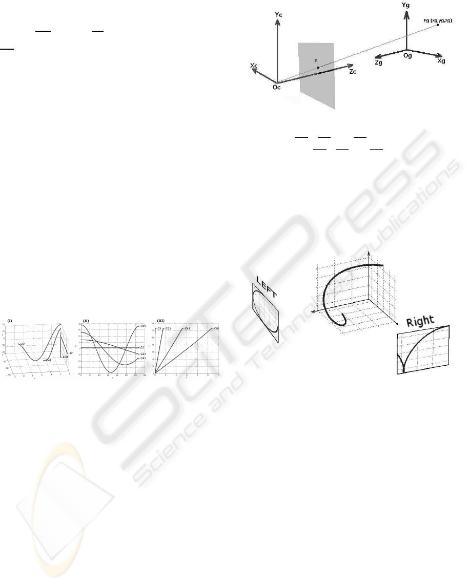
Figure 2: (I) Samples of the family of helixes obtained by
Eq. (19). (II) View of curves from ZY plane. (III) And view
from XY plane.
4.2 Images Acquisition System
A sufficient number of points of the mathematical
curve is generated and projected in the respective im-
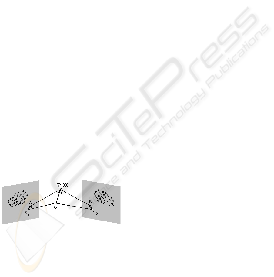
age plane of two virtual pinhole cameras (see Fig. 4).
Both are defined by their respective extrinsic (R and
T) and intrinsic parameters (focal distance, dimen-
sions of pixels, principal point). In terms of geometry,
the extrinsic parameters describe the relation between
the coordinates of a point in global/world P
g
and a
point in the 3D camera system P
c
; here we adopt the
following relation P
g
= RP
c
+T and a geometry such
as that shown in Fig. 3.
By repetition of this process, for various spatial
configurations of the curve, two sets of frames were
consistently created.
Considering the definition of intrinsic and extrin-
sic parameters for both virtual cameras it is possible
Figure 3: The geometry of a pinhole camera model with
image plane in front of the principal point (focus) of the
camera. Axis OX
g
, OY
g
and OZ
g
define the global/world
coordinate system, OX
c
, OY
c
and OZ
c
refer to the camera
system.
to project the points generated by the mathematical
function in both image planes, and right cameras (see
Fig. 4). By repetition of this process for various spa-
tial configurations of the curve two sets of frames are
captured.
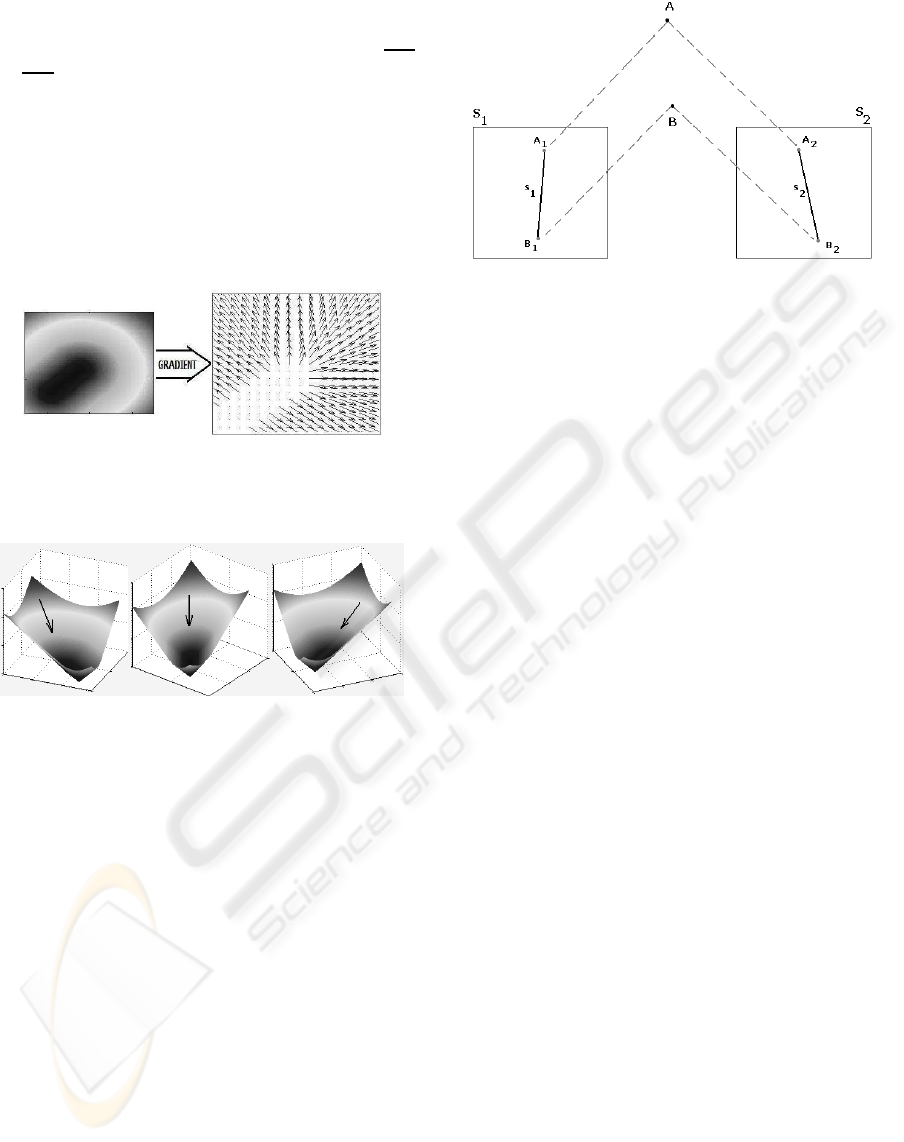
Figure 4: A curve in 3D space has its points projected in a
pair of image planes left and right.
4.3 Vectorial Maps
Provided that the two sequences of frames (from the
left and right cameras) were acquired, the next step is
to transform them in vectorial maps for representing
the external forces components.
Usually, image processing operations are done for
emphasizing features of interest in each frame of the
sequence. At the same time, to prepare the images
to be transformed by a differential operator such as
the gradient. In this work the distance transform is
used in order to generate a matrix whose cells rep-
resents a pixel in the respective frame (image) and
stores the distance from this pixel to the projection of
the curve. Then, this map of distances is operated by
the GVF (Xu and Prince, 1998) originating two ma-
trices with the horizontal and vertical components of
the gradient vectors. For the sake of simplicity, these
two matrices will be considered as just one matrix of
VISAPP 2009 - International Conference on Computer Vision Theory and Applications
550
resultant gradient vectors, which will be called as the
vectorial map associated to its respective frame (im-
age). These maps are responsible for the vectors q
1
A
and q
2
B as shown in Fig. 1. Fig. 5 shows the result of
transformation by distance transform and respective
vectorial map.
Three views of the same distance map could be
seen in Fig. 6, emphasizing its topological attributes
with the feature of interest in the bottom of a valley.
Clearly, there are vectors pointing to (or from) this
valley and they can be extracted by applying a differ-
ential operator.
Figure 5: An image after application of distance transform,
this distance map can be transformed by a gradient operator
in order to get a vectorial map (below).
Figure 6: Three views of a distance map. The map looks
like a geographical valley where the feature of interest lying
on its bottom.
4.4 Automatic Initialization
In its first flash of existence an electrical discharge
usually resembles a straight line linking two points,
similarly its projections look like low curvature
curves. At this moment the discharge can be seen as
an 3D vector whose extremities are points A and B.
This vector can be easily recovered by triangulation
of two pairs of points projected at the pair of images
taken. Such points corresponds to A
1
and A
2
, B
1
and
B
2
in Fig. 7, these are used for triangulation (Trucco
and Verri, 1998) in order to get A and B.
The 3D vector V is defined by V = B − A, and
the set of points C that are generated by this vec-
tor are determined by p = A + cV, where c ∈ R and
0 ≤ c < 1. Geometrically, the set C corresponds to
the reconstruction of the electrical discharge in 3D at
its initial instants of existence. These 3D points are
approximated by a third order B-spline (B
0
) the first
spatial representation of the 3D-snake.
Figure 7: A can be determined by triangulation (Trucco and
Verri, 1998) based on A
1
and A
2
its projections, similarly, B
can be found by triangulation by B
1
and B
2
.It is possible to
triangulate A
1
and A
2
to obtain A, as well as B
1
and B
2
to
obtain B. A and B are extremities of the electrical discharge
in 3D.
4.5 Deformation
The 3D-snake, represented by a B-spline, should de-
form itself according of the minimization of its total
energy functional described in Eq. 1. The snake con-
verges to a stable configuration when a minimum of
energy has been obtained which means that the de-
formation should stop because an equilibrium of the
internal and external forces has been reached. The
goal here is a tracking operation, so the snake needs
to find the equilibrium for each pair of vectorial map
available.
Now, consider the set of i pairs of vecto-
rial maps, where m
j
i
represents a map in ith
time and associated to the jth camera: M =
{(m
1
0
, m
2
0
);(m
1
1
, m
2
1
);...;(m
1
i−1
, m
2
i−1
)}. Also, consider
B
0
as the 3D-snake obtained for the first pair (m
1
0
, m
2
0
).
In order to get the next spatial configurations of the
3D-snake, it is necessary to minimize the functional
in Eq. (1) under the influence of the next pair of maps.
Following such path, the configuration represented by
B
1
results from the evolution of B
0
adjusted to the pair
(m
1
1
, m
2
1
), B
2
results from the evolution of B
1
adjusted
to (m
1
2
, m
2
2
) and so on, up to the (i− 1)th pair of maps
when all of the possible spatial configurations have
been taken in three-dimensional space.
5 RESULTS
The actual lengths of the helixes versus the ones cal-
culated by 3D-snake are shown in Fig. 8. Also, for
each helix the average of its curvature was calculated
and is exhibited in Fig. 9 and the deviation is shown
in Fig. 10.
A NEW APPLICATION FOR 3D-SNAKES - Modelling Electrical Discharges
551
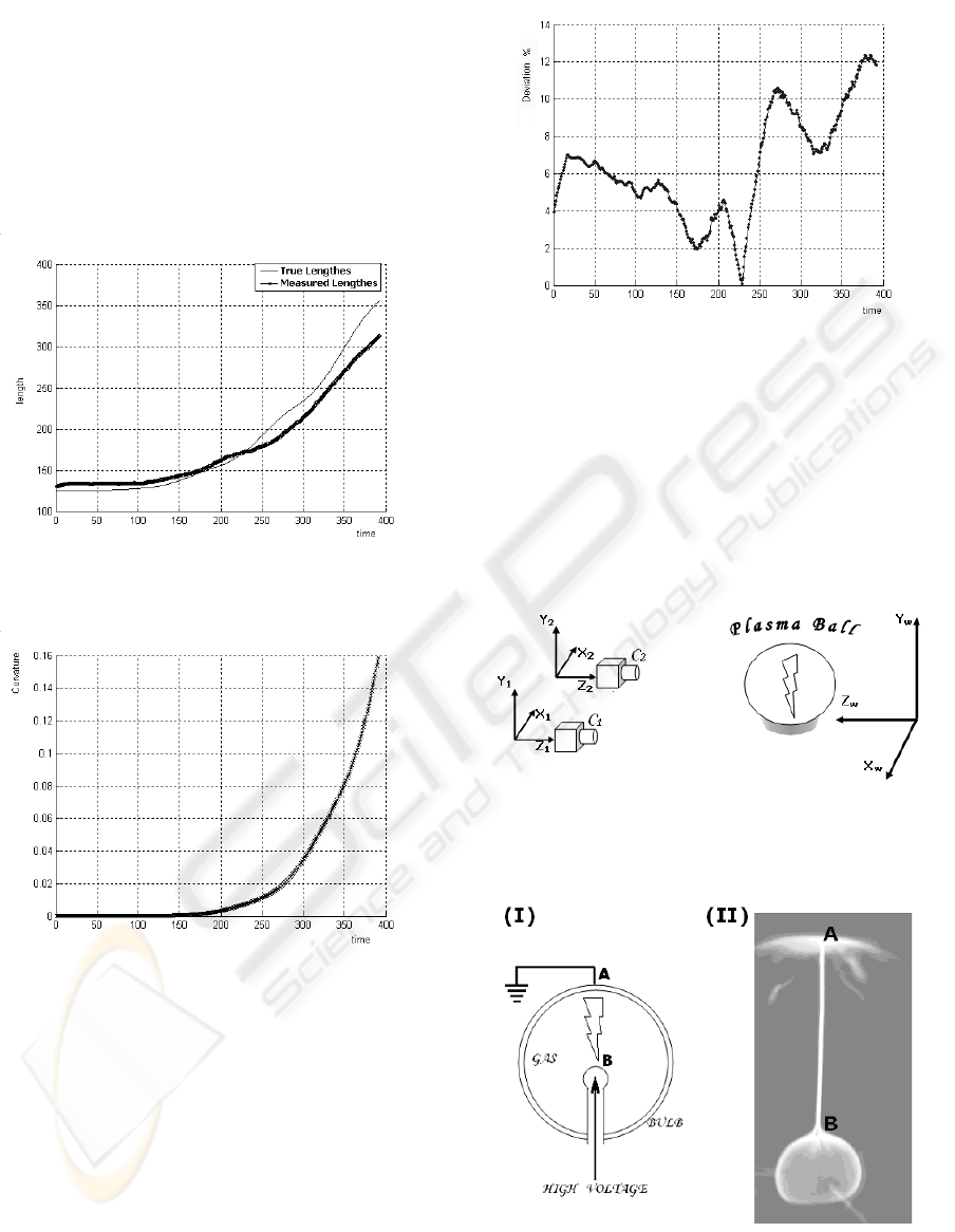
The deviation rises according to the rising of the
curvature of the helixes. On the other hand, the 3D-
snake provides a good estimate for the length of the
electrical discharge, as seen in Fig. 8 the measure-
ments made through the 3D-snake model follow the
profile determined by the actual measurements.
The model works well for medium and low curva-
tures which represents an improvement in comparison
with methods found in the literature .
Figure 8: Real lengthes of the helixes versus lengthes cal-
culated by 3D-snake model.
Figure 9: Real curvature for each helix created by Eq.(19).
5.1 Testing the Proposal with Real
Discharges
Since the approach was validated with sinthetic
curves, it will be applied to real images. A pair of dig-
ital cameras Sony
r
DSC-P200, at 30 fps, was used
to capture the discharge images produced in the ap-
paratus called Plasma Ball driven by capacitive effect
(Fig. 11). The cameras were calibrated by a chess pat-
tern, according Trucco’s method (Trucco and Verri,
1998). The Plasma Ball is a very safe and cheap way
to produce electrical discharges, it is basically a glass
Figure 10: Average deviation for each measured on 3D-
snake.
bulb filled with a special gas and a source of alternat-
ing high voltage (not as high as produced by a Tesla
coil). When the glass bulb is touched, from the out-
side, a bright discharge is generated by the electrical
field produced on that point. The arcs are produced by
the high voltage and the physical effect called capac-
itive force, in regions inside the ampoule where the
gas become more conductive, see Fig. 12.
Figure 11: Acquisition system: C
1
(Sony
r
P100) and C
2
(Sony
r
P200) usual digital cameras. The plasma ball is the
apparatus used for producing the electrical discharges.
Figure 12: (I) Details of the Plasma Ball: distance AB is
d
AB
≈ (60± 0.5)mm. (II) Electrical discharge produced.
A set of image pairs was captured followed by
VISAPP 2009 - International Conference on Computer Vision Theory and Applications
552

the approach proposed to do the measurements of the
discharge, based on the 3D-snake. As an example,
was obtained for the discharge lenghts: ≈ (60.46 ±
0.44)mm. The set of dischargespresents very low cur-
vature, so the distance d
AB
≈ (60 ± 0.5)mm shown in
(Fig. 12) is a good result for the true length, allowing
characterization of the electrical discharges, such as
current density and other electrical parameters.
After these experiments the method will be ap-
plied to high voltage transmission lines.
6 CONCLUSIONS
This work described and validated an approach to be
applied in modelling of electrical discharges captured
in a sequence of stereo pairs. The approach was tested
with an image database built by a consistent strategy
and the cameras were based on the classical theoreti-
cal pinhole camera model.
The results obtained by 3D-snake in estimating
the length of the curves are coherent with the real
lengths. Since the cameras are calibrated it is also
possible to determinate the real position of the electri-
cal discharge during the time of the image acquisition,
so the approach proposed here can work as a strategy
for tracking. A new field of application for 3D active
contours is opened, such as the tracking of electrical
discharges captured in a pair of digital videos and the
study of fast events.
Thus, in the near future this methodology will
be applied in the studies of real electrical discharges
where, certainly, will be found new constraints and
more critical requirements to be evaluated.
ACKNOWLEDGEMENTS
The authors thank the financial support received from
FAPESP - The State of S˜ao Paulo Research, from
CNPq - The National Council for Scientific and Tech-
nological Development and from CAPES - Coordina-
tion of Improvement of Higher Level Education Per-
sonnel. Special thanks to Mr. Marco Iacovacci.
REFERENCES
Amarasinghe, D., Sonnadara, U., Berg, M., and Cooray, V.
(2007). Correlation between brightness and channel
currents of electrical discharges. IEEE Transactions
on Dielectrics and Electrical Insulation, 14(5):1154–
1160.
Amini, A. A., Tehrani, S., and Weymouth, T. E. (1988). Us-
ing dynamic programming for minimizing the energy
of active contours in the presence of hard constraints.
In Second International Conference in Computer Vi-
sion, pages 95–93.
Blake, A. B. and Isard, M. (2000). Active Con-
tours. Springer, 2nd edition. Available at URL:
http://research.microsoft.com/
Canero, C. (2002). 3D Reconstruction of the Coronary Tree
Using Biplane Snakes. PhD thesis, Universitat Aut-
noma de Barcelona, Bellaterra.
Canero, C., Radeva, P., Toledo, R., Villanueva, J. J., and
Mauri, J. (2000). 3d curve reconstruction by biplane
snakes. In Proceedings of the International Confer-
ence on Pattern Recognition (ICPR’00), volume 4,
pages 4563–4566.
Ihlow, A. and Seiffert, U. (2005). Snakes revisited : Speed-
ing up active, contours models using the fast fourier
transform. In Proceedings of the Eighth IASTED In-
ternational Conference : Intelligent Systems and Con-
trol, pages 416–420.
Kass, M., Witkin, A., and Terzopoulos, D. (1988). Snakes:
Active contours models. Second International Con-
ference in Computer Vision, 1(4):321–331.
MacAlpine, J. M. K., Qiu, D. H., and Li, Z. Y. (1999). An
analysis of spark paths in air using 3-dimensional im-
age processing. IEEE Transactions on Dieletrics and
Electrical Insulation, 6(3):331–336.
Qiu, D. H. and MacAlpine, J. M. K. (2000). An incremental
analysis of spark paths in air using 3-dimensional im-
age processing. IEEE Transactions on Dieletrics and
Electrical Insulation, 7(6):758–763.
Qiu, D. H., MacAlpine, J. M. K., and Li, Z. Y. (1999). An
incremental 3-dimensional analysis of spark paths in
air. In Conference on Electrical Insulation and dielet-
ric Phenomena, volume 2, pages 646–649.
Rogers, D. F. and Adams, J. A. (1990). Mathematical Ele-
ments for Computer Graphics. Mc-Graw Hill.
Thevenaz, P. and Unser, M. (2008). Snakuscules. IEEE
Transactions on Image Processing, 17(4):585–593.
Trucco, E. and Verri, A. (1998). Introductory techniques for
3D Computer Vision. Prentice Hall.
Williams, D. J. and Shah, M. (1992). A fast algorithm for
active contours and curvature estimation. In Proceed-
ings of Computer Vision, Graphics, and Image Pro-
cessing, volume 55, pages 14–26.
Xu, C. and Prince, J. L. (1998). Snakes, shapes, and gradi-
ent vector flow. IEEE Transactions on Image Process-
ing, 7(3):359–369.
A NEW APPLICATION FOR 3D-SNAKES - Modelling Electrical Discharges
553
