ACTIVE CONTOURS WITH OPTICAL FLOW AND PRIMITIVE
SHAPE PRIORS FOR ECHOCARDIOGRAPHIC IMAGERY
Ali K. Hamou and Mahmoud R. El-Sakka
Department of Computer Science, University of Western Ontario, London, Ontario, N6A 5B7, Canada
Keywords: Active contours, Deformable models, Snakes, Gradient vector flow, Shape priors, Optical flow,
Echocardiography.
Abstract: Accurate delineation of object borders is highly desirable in echocardiography. Among other model-based
techniques, active contours (or snakes) provide a unique and powerful approach to image analysis. In this
work, we propose the use of a new external energy for a GVF snake, consisting of the optical flow data of
moving heart structures (i.e. the perceived movement). This new external energy provides more information
to the active contour model to combat noise in moving sequences. An automated primitive shape prior
mechanism is also introduced, which further improves the results when dealing with especially noisy
echocardiographic image cines. Results were compared with that of expert manual segmentations yielding
promising sensitivities and system accuracies.
1 INTRODUCTION
Echocardiography, imaging the heart using
ultrasound waves, has become the most widely used
modality to observe heart motion and deformation
over other modalities (e.g. Positron Emission
computed Tomography, Cardiac Magnetic
Resonance, Computer Tomography). This is due to
the relatively inexpensive cost of the technology
along with its non-invasive nature, yielding no
known side-effects. Sophisticated enhancements to
the acquisition devices over the years have yielded
real-time dynamic observation of heart function.
Unfortunately, US data still suffers from speckle
noise. It may also exhibit occluded borders due to
the erratic scattering of its impinging waves (once it
encounters various tissue densities). Efforts have
been made to compensate for these shortcomings,
including filtering (Mazumdar, 2006) and
incorporating the speckle noise effect directly into
the algorithm (Tauber el al., 2008). Regardless,
boundary detection techniques need to be employed
in order to segment a region of interest (ROI).
Analysis of these segmented regions has led to
various works on endocardial borders (Choy and Jin,
1996), stress and strain of the septum (Montagnat
and Delingette, 2000), and wall motility (Amini et
al., 1998), which all help to accurately diagnose
cardiomyopathies.
Many computer vision techniques have been
introduced in order to accomplish boundary
detection. One such example is the active contour
model, also commonly known as snakes (Kass et al.,
1988).
Active contours treat the surface of an object as
an elastic sheet that stretches and deforms when
external and internal forces are applied to it. These
models are physically-based, since their behavior is
designed to mimic the physical laws that govern
real-world objects, (Cohen, 1991). Since this
approach relied on variational calculus to find a
solution, time complexity was a major drawback.
Amini et al. (1990) and Williams and Shah (1992)
proposed algorithms that reduced time complexity
making the active contour model feasible for
segmentation systems.
Issues with large capture ranges (the failure of
curve migration when initialized distant from the
ROI to segment) and concavities (high internal
energies may inhibit the capture of smaller features)
are solved by other advances, which include
inflation forces (Cohen and Cohen, 1993),
robabilistic models (Mallouche et al., 1995),
oriented particles (Szeliski and Tonnesen, 1992),
and gradient vector flows (GVF) (Xu and Prince,
2000). For the purposes of this study, focus will be
placed on those advances best suited for
echocardiographic images.
111
K. Hamou A. and R. El-Sakka M. (2009).
ACTIVE CONTOURS WITH OPTICAL FLOW AND PRIMITIVE SHAPE PRIORS FOR ECHOCARDIOGRAPHIC IMAGERY.
In Proceedings of the First International Conference on Computer Imaging Theory and Applications, pages 111-118
DOI: 10.5220/0001804201110118
Copyright
c
 SciTePress

Since the left ventricle represents one of the most
important heart functions, many semi-automatic
techniques have attempted to segment this region
from its surrounding tissue.
Papademetris et al. (1999) proposed to measure
the stress and strain of cardiac regional deformation
of the left ventricle in ultrasound images by using a
Markov random field (Kindermann and Snell, 1980).
Texture data was incorporated into their model for
use with a tracking algorithm. However,
assumptions of uncorrelated data within their model
are made (which may lead to a misclassification of
structures due to noise) and complex calculations
result in long computation times.
Eusemann el al. (2002) proposed the use of a
modality independent quantitative visualization of
the peak velocities. Though set manually, the
technique utilizes a set of polygon meshes to deform
by means of the anatomical centerline of the left
ventricle.
Jolly (2003) proposed a semi-automatic
segmentation algorithm with the use of three
manually placed landmarks in order to estimate the
location of various shape models. However, this
system was designed for use on the end-systole and
end-diastole images only, rather than the entire
cardiac cycle.
Felix-Gonzalez and Valdes-Cristerna (2006)
proposed a technique using a series of standard
algorithms (e.g. mean shift filtering, edge mapping,
entropy extraction and confidence mapping) along
with an active surface model in order to deal with
the speckle. This model is made up of cubic splines
and is based on gradient descent, however no
explanation is given on parameterization and how
the empirical data was set.
Zhou el al. (2004) proposed the segmentation of
MRI cardiac sequences using a generalized fuzzy
GVF map along with a relative optical flow field.
Optical flow measurements are computed on the
cardiac sequence and a maximum a posteriori
probability (MAP) is used as a window for the
movement of the curve. The use of optical flow with
GVF provides promising results, however since this
technique is used exclusively on MRI data, there is
no guarantee that it would work with US data given
the presence of speckle noise.
In practice, many of the stated segmentation
algorithms can be used on normal echocardiographic
data. This is true given an adequate amount of user
intervention and when such data exhibits low levels
of speckle noise (i.e. from newer machines generally
found in a research environment under ideal
conditions with healthy volunteers). However in a
clinical setting, the objective is to be able to
accurately identify myocardial borders on
problematic echocardiograms with minimal time.
In this paper, we will present an external energy
for GVF snakes that takes advantage of the motion
data within echocardiographic image cines.
Furthermore, we incorporate the use of primitive
shape priors such that the contour placement will
improve, especially when dealing with noisy regions
and improper initialization.
The rest of the paper is organized as follows.
Background information on relevant models will be
briefly described in Section 2. The proposed scheme
will be outlined in Section 3. Section 4 and Section 5
will contain the experimental results and
conclusions, respectively.
2 BACKGROUND
2.1 Active Contours
A snake is an energy minimization problem. Its
energy is represented by two forces (internal energy,
E
in
, and external energy, E
ex
) which work against (or
independent of) each other. The total energy should
converge to a local minimum; ideally at the desired
boundary. A snake can be parametrically defined as
v(s) = [x(s), y(s)]
T
, where s belongs to the interval
[0,1]. Hence, the total energy to be minimized, E
AC
,
to give the best fit between a snake and a desired
object shape is:
∫
+=
1
0
))(())(( dssvEsvEE
exinAC
(1)
where E
in
decreases as the curve becomes smooth
and E
ex
decreases as it approaches the ROI, such as
image structures or edges (i.e. areas of high gradient
information).
As in Kass et al. (1988) the internal energy of the
active contour formulation is further defined as:
2
2
2
2
)()())((
ds
vd
s
ds
dv
ssvE
in
×+×= βα
(2)
where α(s) and β(s) are weighting factors of
elasticity and stiffness, respectively. The first order
term encourages the snake’s surface to act like a
membrane, whereas the second order term
encourages the snake to act like a thin plate. α(s)
controls the tension along the spine (stretching a
balloon or elastic band) whereas β(s) controls the
rigidity of the spine (bending a thin plate or wire).
IMAGAPP 2009 - International Conference on Imaging Theory and Applications
112

(a)
(b)
Figure 1: An example of the virtual electric field; (a)
standard U-Image; (b) virtual electric field of image
shown in (a).
A typical external energy formulation for a given
image, I(x,y), to identify edges is:
2
),(),( yxIyxE
ex
∇−=
(3)
where ∇ denotes the gradient operator. In the case of
a noisier image the edges are further smoothed:
[]
2
),(),(),( yxIyxGyxE
ex
∗∇−=
σ
(4)
where G
σ
(x,y) is a two-dimensional Gaussian
function with standard deviation σ, and ∗ denotes a
convolution operator. σ must be large enough to
compensate for the image noise that would interfere
with the active contour’s capture range (the contour
may get trapped by the noisy areas of the image).
The standard snake algorithm suffers from poor
range due to initialization and the inability to capture
concavities. Xu and Prince (2000) largely solved this
problem by the advent of the GVF snake, which
provides a field for guiding the contour to regions of
high gradient. The GVF field is used as an external
energy and is characterized by the vector field
z(x,y)=[u(x,y),v(x,y)] that minimizes the energy
functional:
∫
∫
∫∫
∇−×∇+
∇+∇×=
dxdyfzf
dxdyvuE
GVF
22
22
||||
)|||(|
μ
(5)
where f
= −E
ex
is an edge map derived from the
image and μ is the degree of smoothness of the field.
Figure 1 shows an example of a GVF field on a
standard U-Image.
2.2 Optical Flow
Optical flow approximates the apparent motion of an
object over a series of images (or time). The
relationship between the optical flow in the image
plane and the velocities of objects in the three
dimensional world is not necessarily obvious
(Barron et al., 1994). For the sake of convenience,
most optical flow techniques consider a particularly
simple world where the apparent velocity of
brightness patterns can be directly identified with the
movement of surfaces in the scene. This implies that
objects maintaining structure but changing intensity
would break this assumption.
Consider an image intensity, I(x,y,t) at time t.
Time, in this instance, implies that next frame in an
image cine. Assuming that at a small distance away,
and some time later the given intensity is:
termsorderhighert
t
I
y
y
I
x
x
I
tyxIttyyxxI
+Δ
∂
∂
+Δ
∂
∂
+Δ
∂
∂
+
=
Δ
+
Δ
+
Δ
+
),,(),,(
(6)
Given that the object started at position (x,y) at
time t, and that it moved by a small distance of (∆x,
∆y) over a period of ∆t, the following assumption
can be made:
),,(),,( tyxIttyyxxI =Δ
+
Δ
+
Δ
+
(7)
The assumption in (7) would only be true if the
intensity of our object is the same at both time t and
t + ∆t. Furthermore, if our ∆x, ∆y and ∆t are very
small, our higher order terms would vanish:
0=Δ
∂
∂
+Δ
∂
∂
+Δ
∂
∂
t
t
I
y
y
I
x
x
I
(8)
Hence dividing (8) by ∆t will yield:
t
y
y
I
t
x
x
I
t
I
Δ
Δ
∂
∂
+
Δ
Δ
∂
∂
=
∂
∂
−
(9)
ACTIVE CONTOURS WITH OPTICAL FLOW AND PRIMITIVE SHAPE PRIORS FOR ECHOCARDIOGRAPHIC
IMAGERY
113

v
y
I
u
x
I
I
t
∂
∂
+
∂
∂
=−
, (10)
where
t
x
u
Δ
Δ
=
and
t
y
v
Δ
Δ
=
.
The equation in (10) is known as the optical flow
constraint equation, where I
t
at a particular pixel
location, (x,y), is how fast its intensity is changing
with respect to time, u and v are the spatial rates of
change for any given pixel (i.e. how fast an intensity
is moving across an image). However, effectively
estimating the component of the flow (along with
intensity values) cannot directly be solved in this
form since it will yield one equation per pixel for
every two unknowns, u and v. In order to do so,
additional constraints must be applied to this
equation.
Horn and Schunck (1981) introduced a method
for solving this problem using partial derivatives. A
global regularization constraint is used which
assumes that images consist of objects undergoing
rigid motion, and so over relatively large areas the
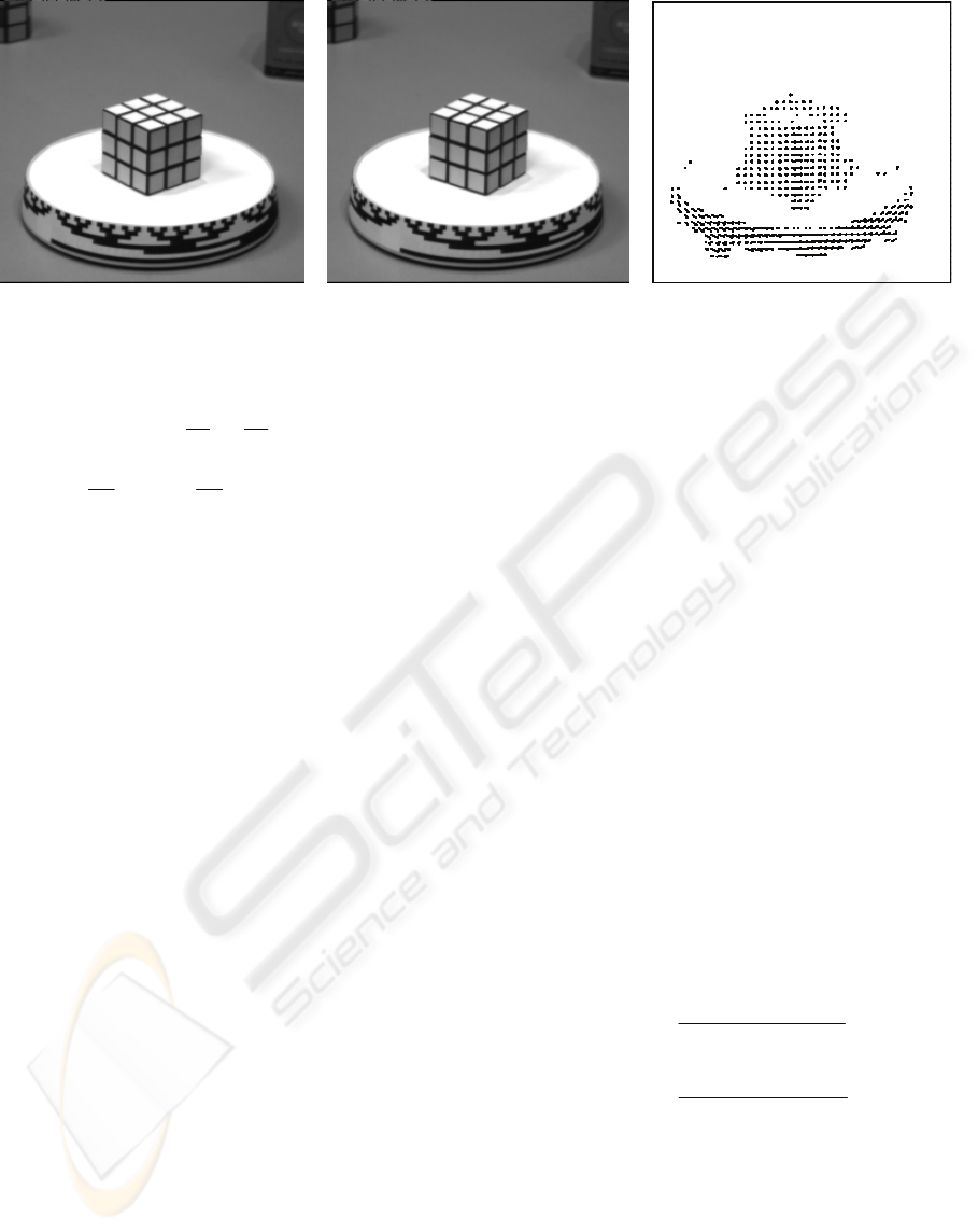
optical flow will be smooth. Figure 2 depicts a
visual representation of the optical flow of a simple
Rubik’s cube. Note that the grayscale image has few
shadows. This helps to maintain consistency in the
luminance of each pixel which in turn yields
accurate results.
3 DESCRIPTION OF PROPOSED
MODEL
The use of the GVF snake directly on
echocardiograms will not provide an adequate
solution due to the complication of noise and other
valves that exist within the heart cavity. Hence our
scheme will make use of a GVF snake with optical
flow measurements. These measurements will be
included in E
GVF
.
By considering each image cine within an
echocardiographic video loop, the Horn-Schunck
technique is applied in order to detect the motion
between various heart structures. These optical flow
measurements will further filter noise from the cines
since speckle tends to be stable throughout an image.
As such, noise will be assigned smaller magnitudes
of movement over surrounding structures and hence
will be eliminated.
The magnitude of these optical flow estimates
are then median filtered and the canny edge map
(Canny, 1986) is extracted in order to generate the
GVF field for the snake’s external energy.
Since the generation of the GVF field is
computationally prohibitive using real world data,
the external energy is generated using a virtual
electric field (VEF) of the preprocessed edge map
(Park and Chung, 2002). The VEF is defined by
considering each edge as a point charge within an
electric field. This can be accomplished by
convolving the edge map with the following two
masks:
2/322
)(4
),(
yx
x
yxg
x
+×
−
=
πε
(11)
2/322
)(4
),(
yx
y
yxg
y
+×
−
=
πε
(12)
where
ε is sufficiently small. Given a sufficient
mask size, the resulting field yields a vector flow
identical to the GVF field defined in (5), without the
high computational cost. For instance, the vector
field shown in Figure 1 was generated with (11) and
(12) with a mask size of 32.
Since many of the anatomical structures (such as
the left ventricle of the heart) are known shapes and
(a) (b) (c)
Figure 2: An example of an optical flow field on a Rubik’s cube rotated image; (a) Rubik’s cube at time t; (b) Rubik’s
cube at time t+∆t; (c) optical flow.
IMAGAPP 2009 - International Conference on Imaging Theory and Applications
114

sizes, prior knowledge information can be directly
used to increase the performance of a segmentation
algorithm.
Priors based on shape statistical models require
modifications to the standard active contour model.
An iterative solution can be directly incorporated
into any optimization model by using the proposed
framework first outlined by Hamou et al. (2007).
Since it is desirable to incorporate shape priors
into the model without directly involving the user,
automated shape detection takes place on the set of
discrete snake points, v(s). This is achieved by
replacing E
ex
of our active contour with a least
squares fit polynomial (specifically a third order
hyperbola) of the current v(s) points. This allows the
fitting of a primitive shape (or a series of primitives
as needed for the left ventricle) to the curve set v(s).
This will help compensate for the noise that inhibits
the snake from migrating past a certain point. The
user is able to increase or decrease the effect of the
prior knowledge to the snake’s convergence cycle.
Depending on the feature of interest to be
segmented, different primitive priors can be used in
order to improve the robustness of the technique.
The priors are not limited to hyperbolas; rather a
range of shapes can be selected by the user in order
to best fit their feature of interest. This is useful in
the medical arena where a specialist has a clear
understanding of the underlying structure being
detected, such as a liver, an artery, or a heart. A
desired primitive shape can be selected before curve
evolution takes place.
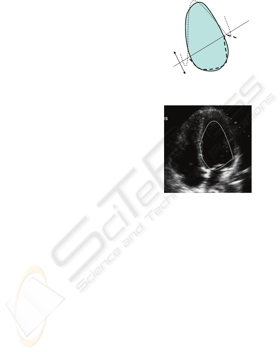
Figure 3 portrays the means of generating a
primitive prior for the left ventricle of the 4 chamber
view US heart image. The left ventricle points were
split into an upper region and a lower region
representing two separate shape fitting equations.
This can be tuned to give the best prior by selecting
the separation line of the regions with the least
amount of distance between the fitted hyperbolas
and snake curve. Further advantages are that the
prior knowledge is not built on a set of training
samples that are expert delineated; rather they are
generated from the current active contour control
points. Figure 4 shows the results of the prior
generation scheme on a echocardiogram.
Once the prior is constructed, a VEF is generated
of the prior and a single optimization iteration of the
snake is executed before returning to the original
optimization cycle. This is referred to as an omega
iteration. This interruption to the snake optimization
cycle is repeated throughout the snake’s evolution,
until it achieves equilibrium. A flow chart of the
proposed scheme is shown in Figure 5.
4 EXPERIMENTAL RESULTS
For this study, a series of B-mode echocardiogram
cross sectional videos of the heart have been used to
investigate the proposed snake algorithm. These
videos were acquired using a SONOS 5500 by
Philips Medical System. The transducer frequency
was set at 2.5 Mhz in order to insure adequate
penetration of tissue, while maintaining image
quality with the existing speckle noise. Longitudinal
views of the heart, which visualize the left ventricle,
were acquired in order to verify the prior knowledge
algorithm using more than one primitive shape.
2/3 upper region
1/3 lower region
Snake of
LV
Shift in order
to attain
optimal prior
Figure 3: Generation of primitive priors on active contour
points.
Figure 4: An example of a primitive prior formulation on
the left ventricle.
ACTIVE CONTOURS WITH OPTICAL FLOW AND PRIMITIVE SHAPE PRIORS FOR ECHOCARDIOGRAPHIC
IMAGERY
115

The videos were parsed into image cines and
each frame was considered with its direct
neighbouring frame. Optical flow calculations for
the edge map were completed using the Horn-
Schunck technique with a regularization constraint
of 0.05 in order to compensate for the general
speckle throughout the US images. Mask size for
VEF generation was set to 64 and was normalized
for active contour use. The initial contour placement
was set to a circle of radius 30, which was placed by
the user within the left ventricle of the heart.
Snake parameters,
α and β , were set to 4 and 0,
respectively.
α was set to 4 in order to add a
substantial amount of weight to the internal energy.
β was set to 0 since the second order differential
does not influence the snake enough to warrant the
added time complexity. Priors (omega iteration)
were invoked every five iterations of the snake
minimization.
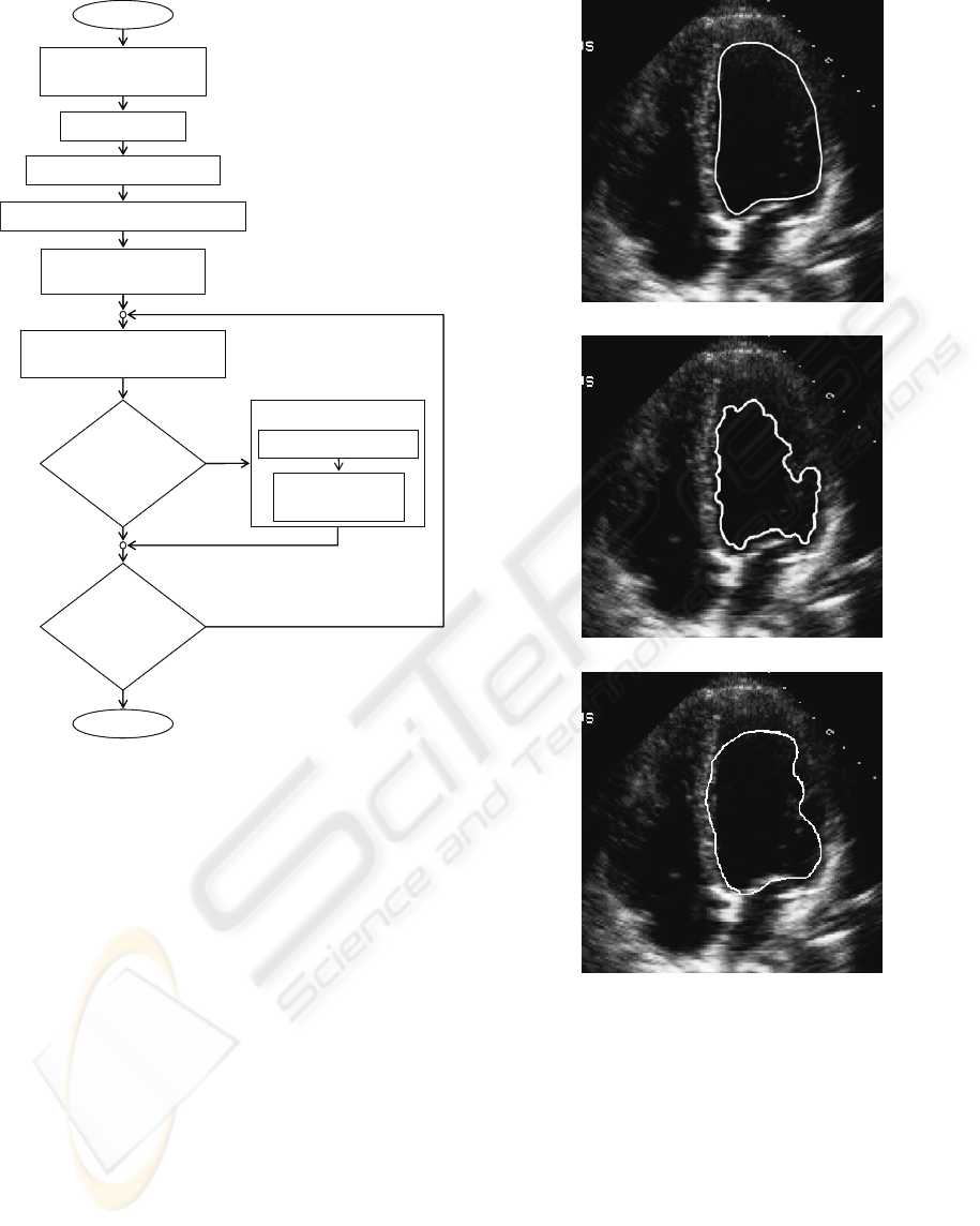
Figure 6(a) shows an expert manual
segmentation of the left ventricle of the heart. Figure
6(b) shows the final contour using the traditional
(a)
(b)
(c)
Figure 6: Segmenting the left ventricle of the heart; (a)
Expert manual segmentation (b) standard GVF
segmentation (c) GVF-optical flow segmentation with
priors.
GVF snake. Figure 6(c) shows the final contour
using the optical flow GVF snake with primitive
priors. Expert examination of the results reveals that
the shape priors improve regularity by allowing the
snake to overcome noise, artifacts. This allows for
proper delineation of the left ventricular endocardial
lining. The optical flow measurements provide the
necessary structural information used in the external
Calculate Virtual Electric Field E
ex
Calculate Magnitude
of Optical Flow
Snake Initialization
(Seed Point)
Iterate snake to further
minimize energy
Stop
Omega
cycle
detected
Generate Canny Edge Map
Preprocessing
Start
Stopping
criteria not
met?
(Isolated E
ex
)
Calculate Shape Prior
Generate Virtual
Electric Field
Yes
Yes
No
No
Calculate Virtual Electric Field E
ex
Calculate Magnitude
of Optical Flow
Snake Initialization
(Seed Point)
Iterate snake to further
minimize energy
Stop
Omega
cycle
detected
Generate Canny Edge Map
Preprocessing
Start
Stopping
criteria not
met?
(Isolated E
ex
)
Calculate Shape Prior
Generate Virtual
Electric Field
Yes
Yes
No
No
Figure 5: Flow Chart of Proposed Algorithm.
IMAGAPP 2009 - International Conference on Imaging Theory and Applications
116

energy of the snake.
Experiments were run on a complete cardiac
cycle with various external energies. The first
consisting purely of the optical flow measurements,
the second on a combined energy of image gradient
vectors and optical flow data.
Overall, accuracy of the proposed system was
measured by comparing the 87 indexed images to
the expert manual segmentations by a clinician.
These measurements include both type I and type II
errors as defined by Neyman and Pearson (1928).
Since the images were mainly small segmented
foregrounds against vast backgrounds, the system
would best be measured by means of its sensitivity
and system accuracy.
Sensitivity is the number of true positives
divided by the number of true positives plus false
negatives. System accuracy is the number of true
positives and true negatives divided by the total
number of pixels in the image. In other words, it
classifies how accurate the results of the test are
versus the total image.
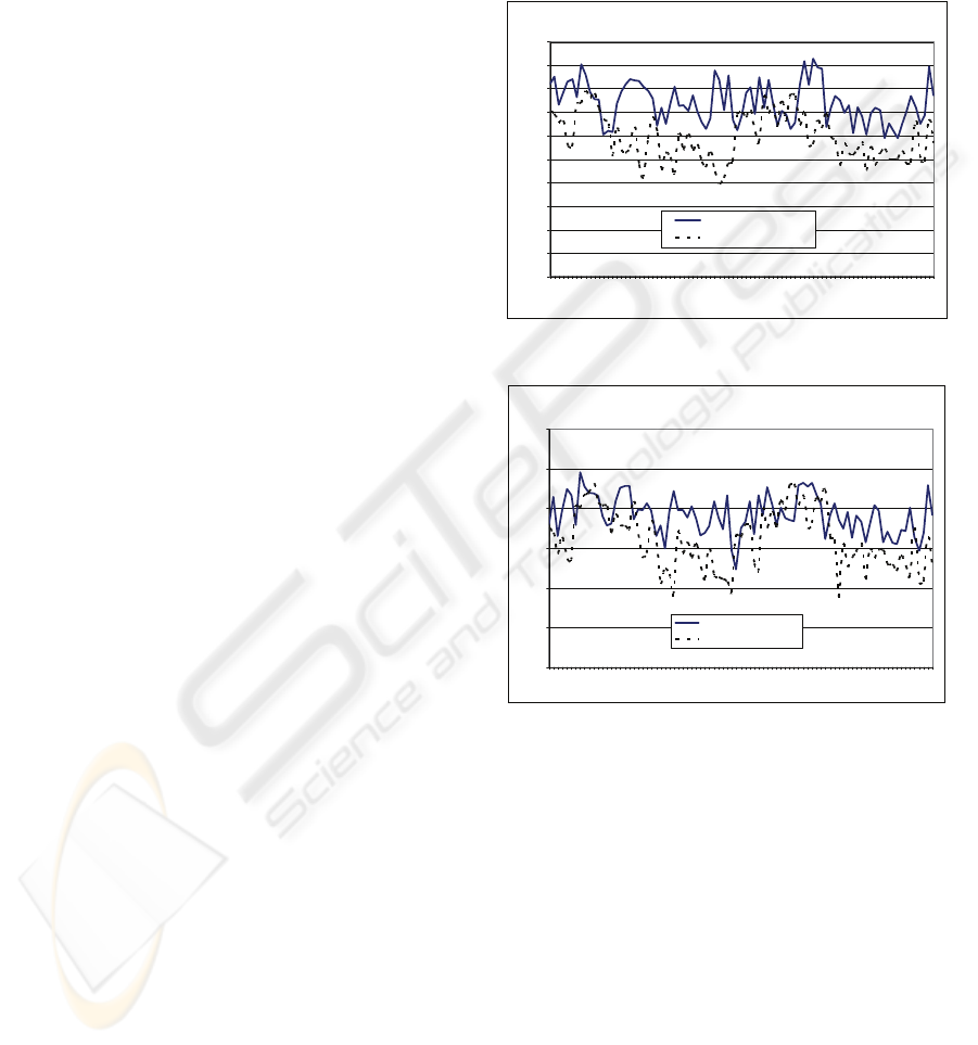
The sensitivity of the system, given a 95%
confidence interval, yields 0.568-0.610 when using
the optical flow exclusively. However this yield
increased to 0.722-0.759 when combined with a
image gradient vectors. Whereas, system accuracy,
given the same confidence interval, yields 0.940-
0.946 for the optical flow energy and 0.954-0.958
for the combined energy, respectively.
Figure 7 shows the sensitivity of the system
using various energies. Figure 8 shows the system
accuracy of the system. We notice that there is a
slight improvement when segmenting using both the
optical flow and the image gradient over the optical
flow exclusively. This illustrates that the optical
flow measurements contributes enough information
to the snake in order to segment out the left
ventricle.
5 CONCLUSIONS
In this paper, we have shown that the use of optical
flow calculations can be used as an external energy
within the GVF active contour framework. By
exclusively using the optical flow calculations, we
have shown that it is possible that an active contour
method can make use of the knowledge derived
from the apparent motion of tissue. This strengthens
the principle that the movement of tissue masses
should be considered within segmentation
techniques, where the data facilitates it.
Furthermore, contour regularity and accuracy
was improved by using primitive shapes priors. The
inherent difficulties in segmenting echo-
cardiographic images, such as avoiding speckle
noise and valve interference were also overcome by
the primitive priors. Results were validated against a
gold standard which was manually segmented by a
clinician.
0
0.1
0.2
0.3
0.4
0.5
0.6
0.7
0.8
0.9
1
1 4 7 10131619222528313437404346495255586164677073 76798285
Image Index
Sensititivity…
.
Gradient and Optical Flow
Optical Flow
Figure 7: Sensitivity using different external energies.
0.88
0.9
0.92
0.94
0.96
0.98
1
1 4 7 1013161922252831343740434649525558616467707376798285
Image Index
System Accurac
y
….
.
Gradient and Optical Flo
w
Optical Flow
Figure 8: System Accuracy using different external
energies.
ACKNOWLEDGEMENTS
This research is partially funded by the Natural
Sciences and Engineering Research Council of
Canada (NSERC). This support is greatly
appreciated.
REFERENCES
Amini, A., Radeva, P., Elayyadi, M. and Li, D. 1998,
‘Measurement of 3D motion of myocardial material
points from explicit B-surface reconstruction of tagged
ACTIVE CONTOURS WITH OPTICAL FLOW AND PRIMITIVE SHAPE PRIORS FOR ECHOCARDIOGRAPHIC
IMAGERY
117

MRI data’, Medical Image Computing and Computer-
Assisted Intervention, pp. 110-118.
Amini, A., Weymouth, T., and Jain, R. 1990, ‘Using
dynamic programming for solving variational
problems in vision’, IEEE Pattern Analysis in
Machine Intelligence, vol. 12, no. 9, pp. 855-866.
Barron, J., Fleet, D. and Beauchemin, D. 1994,
‘Performance of optical flow techniques’,
International Journal of Computer Vision, vol. 12, no.
1, pp. 43-77.
Canny, J. 1986, ‘A computational approach to edge
detection’, IEEE Pattern Analysis in Machine
Intelligence, vol. 8, no. 6, pp. 679-698.
Choy, M. and Jin, J. 1996, ‘Morphological image analysis
of left ventricular endocardial borders in 2D
echocardiograms’, SPIE Proceedings on Medical
Imaging, vol. 2710, pp. 852-864.
Cohen, I. 1991, ‘On active contour models and balloons’,
Image Understanding, vol. 53, no. 2, pp. 211-218.
Cohen, L. and Cohen, I. 1993, ‘Finite-element methods for
active contour models and balloons for 2-d and 3-d
images’, IEEE Transactions on pattern analysis and
Machine Intelligence, vol. 15, no. 11, pp. 1131-1147.
Eusemann C., Ritman E. and Robb R. 2002, ‘3D
visualization of endocardial peak velocities during
systole and diastole’, Medical Imaging: Physiology
and Function from Multidimensional Images, vol
4683, pp. 168-175.
Felix-Gonzalez, N. and Valdes-Cristerna R. 2006, ‘3D
echocardiographic segmentation using the mean-shift
algorithm and an active surface model’, SPIE Medical
Imaging 2006: Image Processing, vol. 6144, pp. 1314-
1319.
Hamou, A., Osman, S. and El-Sakka, M., 2007, ‘Carotid
ultrasound segmentation using DP active contours’,
International Conference on Image Analysis and
Recognition, vol. 4633, pp. 961-971.
Horn, B. and Schunck, B. 1981, ‘Determining optical
flow’, Artificial Intelligence, vol. 17, pp. 185-203.
Jolly, M. 2006, ‘Assisted ejection fraction in B-mode and
contrast echocardiography’, Biomedical Imaging:
Nano to Macro, pp. 97-100.
Kass, M., Witkin, A. and Terzopoulos, D. 1988, ‘Snakes:
Active contour models’, International Journal of
Computer Vision, vol. 1, no. 4, pp. 321-331.
Kindermann, R and Snell, J. 1980, Markov random fields
and their applications, American Mathematical
Society, Providence, R.I.
Mallouche, H., de Guise, J. and Goussard, Y. 1995,
‘Probabilistic model of multiple dynamic curve
matching for A semitransparent scene’, SPIE Vision
Geometry IV, vol. 2573, pp. 148-157.
Mazumdar, B., Mediratta, A., Bhattacharyya, J. and
Banerjee, S. 2006, ‘A real time speckle noise cleaning
filter for ultrasound images’, IEEE Symposium on
Computer-Based Medical Systems, pp. 341-346.
Montagnat, J. and Delingette, H. 2000, ‘Space and time
shape constrained deformable surfaces for 4D medical
image segmentation’, Medical Image Computing and
Computer-Assisted Intervention, vol. 1935, pp. 196-
205.
Neyman, J. and Pearson, E. 1928, ‘On the use and
interpretation of certain test criteria for purposes of
statistical inference, part I’, Biometrika, vol. 20a, no.
1/2, pp. 175-240.
Papademetris, X., Sinusas, A., Dione, D. and Duncan, J.
1999, ‘3D cardiac deformation from ultrasound
images’, Medical Image Computing and Computer-
Assisted Intervention, vol. 1679, pp. 420-429.
Park, H. and Chung, M. 2002, ‘A new external force for
active contour model: virtual electric field’,
Visualization, Imaging, and Image Processing, vol.
364, pp. 90-94.
Szeliski, R. and Tonnesen, D. 1992, ‘Surface modeling
with oriented particle systems’, SIGGRAPH Computer
Graphics, vol. 26, no. 2, pp. 185-194.
Tauber, C., Batatia, H. and Ayache, A. 2008, ‘Robust B-
spline snakes for ultrasound image segmentation’,
Springer Journal of Signal Processing Systems.
Williams, D. and Shah, M. 1992, ‘A fast algorithm for
active contours and curvature estimation’, CVGIP:
Image Understanding, vol. 55, no. 1, pp. 14-26.
Xu, C. and Prince, J. 2000, ‘Gradient vector flow
deformable models’, Handbook of Medical Imaging,
pp. 159-159.
Zhou, S., Liangbin and Chen, W. 2004, ‘A new method
for robust contour tracking in cardiac image
sequences’, IEEE Biomedical Imaging: Nano to
Macro, vol. 1, pp. 181-184.
IMAGAPP 2009 - International Conference on Imaging Theory and Applications
118