RECOVERY OF THE RESPONSE CURVE OF A DIGITAL IMAGING
PROCESS BY DATA-CENTRIC REGULARIZATION
Johannes Herwig and Josef Pauli
Fakult¨at f¨ur Ingenieurwissenschaften, Abteilung f¨ur Informatik und Angewandte Kognitionswissenschaft
Universit¨at Duisburg-Essen, Bismarckstraße 90, 47057 Duisburg, Germany
Keywords:
Sensor modeling, Sensitometry, Photometric calibration, High dynamic range imaging, Image fusion, Image
acquisition, Radiance mapping, Image segmentation.
Abstract:
A method is presented that fuses multiple differently exposed images of the same static real-world scene into
a single high dynamic range radiance map. Firstly, the response function of the imaging device is recovered,
that maps irradiating light at the imaging sensor to gray values, and is usually not linear for 8-bit images. This
nonlinearity affects image processing algorithms that do assume a linear model of light. With the response
function known this compression can be reversed. For reliable recovery the whole set of images is segmented
in a single step, and regions of roughly constant radiance in the scene are labeled. Under- and overexposed
parts in one image are segmented without loss of detail throughout the scene. From these segments and a
parametrization of digital film the slope of the response curve is estimated, whereby various noise sources of
an imaging sensor have been modeled. From its slope the response function is recovered and images are fused.
The dynamic range of outdoor environments cannot be captured by a single image. Valuable information gets
lost because of under- or overexposure. A radiance map overcomes this problem and makes object recognition
or visual self-localisation of robots easier.
1 PROBLEM OUTLINE
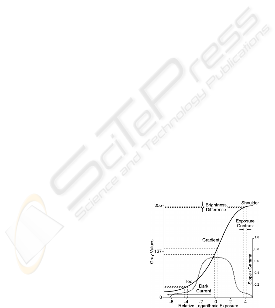
When a photographic film is exposed to irradiating
light E for an exposure time ∆t the emulsion con-
verts the exposure E∆t into contrast (Sprawls, 1993).
The same principle is applicable in analog-to-digital
conversion (ADC) of energy, measured by a charge-
coupled device (CCD) array of a digital imaging de-
vice, to gray values of pixels. Both processes can be
described by the response function shown in figure 1.
In order to produce visually pleasing pictures of low
dynamic range (LDR) made from real-world scenes
of high dynamic range (HDR) the quantization of en-
ergy resulting from irradiating light is usually not pro-
portional (Manders and Mann, 2006).
Then there is no linear mapping of irradiance to
gray values of pixels.
But naturally the mapping of light energy should
be linear, so that any gray value, that is twice as large
as some other, corresponds to twice as much irradiat-
ing light. Most image processing algorithms assume
a linear mapping, but because of HDR to LDR com-
pression this is not valid. E.g. the linear model of light
in shape from shading leads to incorrect results, if
nonlinearities introduced by the imaging sensor have
Figure 1: Semi-log plot of a response curve and its slope.
539
Herwig J. and Pauli J. (2009).
RECOVERY OF THE RESPONSE CURVE OF A DIGITAL IMAGING PROCESS BY DATA-CENTRIC REGULARIZATION.
In Proceedings of the Fourth International Conference on Computer Vision Theory and Applications, pages 539-546
DOI: 10.5220/0001804705390546
Copyright
c
SciTePress

been ignored. Because of lower contrast resolution
in darker or lighter parts of an image, segmentation
algorithms may lead to biased results in regions of a
scene with inhomogeneous lighting: The same gray
value threshold comprises a much wider range of light
values when applied to darker or lighter image areas
than within mid-range gray values. Here an algorithm
is developed that recovers the response function that
is applied to energy of irradiating light by an ADC.
Then the knowledge of the response curve is used
to reverse the compression. This makes thresholds be-
have homogeneouslywithin all ranges of pixel values.
It can support machine vision tasks on assembled ob-
jects of materials with different reflectance properties.
Also object recognition in outdoor environments may
require high contrast within the whole range of pixel
values when only the shape of the object is known but
lighting conditions do vary widely. Shape from shad-
ing could be made more reliable because of reduced
noise, higher precision of pixel values and the linear
model of light.
2 PREVIOUS WORK
Many algorithms for recoveringthe response function
of an imaging processs from a set of differently ex-
posed pictures of the same static scene have been de-
veloped. With the response function known, multi-
ple LDR images taken with varying exposure, usually
with a digital resolution of 8-bit, can be fused into a
single HDR radiance map with 32-bit floating-point
resolution. The method developed in (Debevec and
Malik, 1997) and the one in (Robertson et al., 2003)
are the most widely used.
All three methods do make the same key assump-
tions on the imaging sensor.
1. Uniform response. Each sensor element of the
given imaging device corresponding to one pixel
in the image has equal properties. The ADC be-
haves the same for every pixel.
2. Static response. For every exposure within a se-
quence the same response function is applied.
3. Gaussian noise. Sensor noise is modeled as a nor-
mal distribution and is independent of time and
working environment.
But most of these assumptions do not hold in reality.
1. Non-uniform response. Sensor elements do not
respond uniformly, because of fabrication issues,
vignetting, varying temperature or spatially differ-
ent post-processing in ADC.
2. Adaptive response. Because of automatic color
balancing, automatic film speed adoption and aut-
ofocus, different response functions may be used
for each image within a single exposure series.
3. Non-gaussian noise. Noise is not independent,
because of hot or dead sensor elements, blooming
effects, varying analog gain, cosmic rays, atmo-
sphere and changing transmittance, spatially dif-
ferent post-processing, color interpolation by the
Bayer pattern, integrated circuits, etc.
The algorithm presented in (Mann and Picard, 1995)
was the first, but is not considered to produce satis-
fying results. There no specific error model has been
developed, but instead the response curve is strictly
parametrized and sparse data points obtained from
pixel locations are used for curve fitting.
In (Debevec and Malik, 1997) the response func-
tion is parametrized by a system of linear equations.
A simplistic sensor model is incorporated where gray
values in their mid-range get higher confidence, be-
cause as suggested by figure 1 there the slope of the
response curve is supposed to be large and hence ac-
curacy of measurements is high. Vignetting effects
are neglected because of their small impact. The pixel
locations that serve as an input for their algorithm
have been chosen manually by a human expert to be
free from optical blur.
The error model in (Robertson et al., 2003) is ex-
plicitly gaussian and they justify this by arguing that
noise sources do vary that much, that in its sum it
may be seen as gaussian. Otherwise their basic obser-
vation model is comparable to (Debevec and Malik,
1997), although their approach is probabilistic. There
and also in (Mann and Picard, 1995) the then known
slope of the recovered response curve has been used
to measure confidence when merging irradiance val-
ues of different exposures for the final HDR image.
None of these algorithms does address adaptive
control of the response function during an exposure
series by autocalibration techniques of the imaging
device. The response function has been treated as
constant by all previously introduced reconstruction
methods. The probabilistic method proposed in (Pal
et al., 2004) is capable of this and estimates a different
response function for each input image
An iterative algorithm with an emphasis on sta-
tistical error modeling is given in (Tsin et al., 2001).
Therein some noise sources are ignored because they
are assumed to be constant over all exposures. Ev-
ery valid pixel, e.g. pixels suspected to blooming are
sorted out, is used for computation.
Another iterative method is given in (Mitsunaga
and Nayar, 1999) where the response function is di-
rectly parametrized using a high-order polynomial.
VISAPP 2009 - International Conference on Computer Vision Theory and Applications
540

For recovery its order and coefficients are to be deter-
mined. Their approach has an exponential ambiguity
and the number of solutions is theoretically infinite.
They do assume gaussian noise and only have an
explicit error model for vignetting.
An automated system for recovering the response
curve utilizing Debevec’s algorithm is described in
(O’Malley, 2006). Therein the problem of selecting
unbiased pixel locations free from non-gaussian noise
for an input to Debevec’s linear equations is addressed
by randomly choosing pixel coordinates. Locations
that are most probably prone to errors have been re-
jected afterwards. Specifically only locations with
gray values are accepted that lie within some prede-
fined range within most of the exposed pictures.
In this paper the focus is on non-iterative methods
with a minimum set of input values. Thereby noise
sources are modeled by proper segmentation of the
input scene. In an analytic approach only a small sub-
set of pixel locations is to be chosen as an input of the
algorithm in order to reduce computational effort.
2.1 Recovering the Response Curve
The algorithm for the recovery of the response func-
tion presented in this paper is heavily based on (De-
bevec and Malik, 1997), where a linear system of
equations is proposed. Thereby the exposure time
is known for every photograph. The scene captured
is thought to be composed of mostly static elements,
and changes in lighting during the process should be
neglectable. Basically the idea is that any variation
in pixel values at the same spatial location over the
whole set of images is only due to changed exposure
time.
Now, their method is briefly reviewed.
The physical process that converts exposure E∆t
into discrete gray values Z is modeled by an unknown
nonlinear function f,
Z
ij
= f(E
i
∆t
j
) (1)
Here index i runs over the two-dimensional pixel lo-
cations and j depicts the exposure time. It is assumed
that f is monotonic and therefore invertible,
f
−1
(Z
ij
) = E
i
∆t
j
(2)
Taking the logarithm on both sides, one gets
ln f
−1
(Z
ij
) = lnE
i
+ ln∆t
j
:= g(Z
ij
) (3)
The function g and the E
i
’s are to be estimated. Equa-
tion (3) gives rise to a linear least squares problem.
Only the Z
ij
and ∆t
j
are known, irradiances E
i
are
completely unknown and g at most can only be inves-
tigated at discrete points Z ranging from Z
min
= 0 to
Z
max
= 255. Despite that, g is a continuous curve, and
it maps the Z
ij
’s to the much wider ℜ
+
= [0, ∞) space
of light. For an ill-posed problem a suitable regular-
ization term exploiting some known properties of g is
needed, where g is constrained by a smoothness con-
dition,
O =
N
∑
i=1
P
∑
j=1
[w
z
(Z
ij
)(g(Z
ij
) − lnE
i
− ln∆t
j
)]
2
+
λ
Z
max
−1
∑
z=Z
min
+1
h
w
z
(z)g
′′
(z)
i
2
(4)
where w
z
is a weighting function approximating the
expected slope of the curve, N is the amount of spa-
tially different pixels, and P is the number of differ-
ently exposed images. Without deeper insight into
any specific problem the discrete second derivative
operator is widely used as a regularization term. The
factor λ weights the smoothness term relative to the
data fitting term. The E
i
’s do constrain the model only
and are later computed by equation (5) more accu-
rately. Finally when the response function g is known,
the rearranged equation (3) is used to solve for the
irradiance values E
i
and the final radiance map. To
reduce noise its the weighted average over all images
lnE
i
=
∑
P
j=1
w
z
(Z
ij
)(g(Z
ij
) − ln∆t
j
)
∑
P
j=1
w
z
(Z
ij
)
(5)
2.2 Empirical Law for Film
The aim of this paper is to develop a method that
makes weaker assumptions on the curve to be recov-
ered. Especially its slope should not be constrained
by a predefined weighting function as in the regular-
ization term of equation (4). Therefore the slope is to
be estimated by the first derivative which has strong
relation to the underlying data in terms of gray val-
ues produced by the imaging sensor itself. In (Mann
and Picard, 1995) the empirical law for film is given,
which parametrizes the response function
f(q) = α+ βq
γ
(6)
where q denotes the amount of irradiating light. With
α the density of unexposed film is denoted, and β is
a constant scaling factor. Two exposures of the same
static scene with no change in radiance are related by
b = k
γ
a (7)
where a and b are gray values of a pixel at the same
spatial location in both images, and where k is the
ratio of exposure values of the images. Suppose that
pixels b of the second image have been exposed to k-
times as much irradiating light as their corresponding
pixels a of the first image. In both equations γ is the
slope of the response curve.
RECOVERY OF THE RESPONSE CURVE OF A DIGITAL IMAGING PROCESS BY DATA-CENTRIC
REGULARIZATION
541

2.3 Graph-Based Segmentation
To estimate the slope of the response curve from pixel
data and to select reliable pixel locations as an input
for the data fitting term in equation (4), the image se-
ries is to be segmented into regions of roughly con-
stant radiance to reduce the impact of the aforemen-
tioned noise sources. For segmentation of all images
of an exposure series in a single step the graph-based
segmentation algorithm developed in (Felzenszwalb
and Huttenlocher, 2004) has been utilized. The algo-
rithm works in a greedy fashion, and makes decisions
whether or not to merge neighboring regions into a
single connected component. The following gives an
outline of their approach.
A graph G = (V, E) is introducedwith vertices v
i
∈
V, the set of pixels, and edges (v
i
, v
j
) ∈ E correspond-
ing to pairs of an eight-neighborhood. Edges have
nonnegative weights w((v
i
, v
j
)) corresponding to the
gray value difference between two pixels. The idea
is, that within a connected component, edge weights,
as a measure of internal difference, should be small
and that in opposition edges defining a border be-
tween regions should have higher weights. If there
is evidence for a boundary between two neighbour-
ing components, the comparison predicate evaluates
to true,
D(C
1
,C
2
) =
(
true, Dif(C
1
,C
2
) > MInt(C
1
,C
2
)
false, otherwise
(8)
where Dif(C
1
,C
2
) denotes the difference between
two components C
1
,C
2
⊆ V, and MInt(C
1
,C
2
) is the
minimum internal difference of both components.
3 THE ALGORITHM
The herein proposed algorithm for creating a HDR
image comprises the following steps:
1. Segment the scene into maximal regions of lim-
ited gray value variance.
2. Select high quality regions of smallest variances
that are evenly distributed over the whole range of
gray values and of a minimum size.
3. Iterate all regions of weaker quality and estimate
the slope of the response curve at every discrete
gray value.
4. Reconstruct the response curve from a small set
of high quality regions for data fitting and use the
estimated slope for regularization.
5. Fuse all exposures into a single radiance map us-
ing the reconstructed response curve.
It is computationally infeasible to minimize the ob-
jective function (4) over all pixels. A number of
promising locations needs to be selected that are most
favourable to achieve an unbiased result. Those loca-
tions should track gray values only that have strongest
correlation to scene radiance and are preferably by
no means disturbed by any source of non-gaussian
noise. An optimal solution for the selection problem
in a greedy sense is proposed here with graph-based
segmentation over all images of an exposure series at
once.
Thereby regions that do provide useful LDR infor-
mation in long exposures only are equally well seg-
mented as parts of the scene for which the opposite is
true. If in one image large parts are overlaid by sat-
urated regions or instead are underexposed missing
information is available in one of the other exposures.
The smoothness term in equation (4), which is
the minimization of the second derivative, is to
be replaced with fitting the first derivative instead.
Whereas no preliminaries are necessary using the sec-
ond derivative, the first derivatives need to be known
in advance. This is accomplished by parametrizing
the pixel response, measured in digital gray values,
by the empirical law for film given in equation (7).
Finally, when the response function has been re-
constructed, the HDR image is created for which all
exposures are fused into a single radiance map.
3.1 Segmentation Over All Images
Producing a single segmentation from a set of images
is regarded as a three dimensional problem with two
dimensional output. This requires an extension in the
weighting of edges,
w
p
((v
i
, v
j
)) = max
(v
ip
,v
jp
)∈{E×P},0<p<P
w((v
ip
, v
jp
)) (9)
Edges are weighted by the maximum gray value dif-
ference between two pixels at spatial locations i and j
in any of the images P of the sequence of exposures.
It is assumed that parts of a scene which are supposed
to be correctly exposed have maximum contrast, be-
cause by definition both under- and overexposed re-
gions in an image have a homogeneous appareance
and therefore lack texture. This w
p
’s replace the orig-
inal edge weights w in the segmentation algorithm.
Therefore a single region can be made up of gray val-
ues obtained from different images of the sequence.
Segmented regions should have a predefined max-
imum variance in gray values only, because image
VISAPP 2009 - International Conference on Computer Vision Theory and Applications
542

regions that have a small intensity variance at their
best exposure are supposed to be robust against opti-
cal blur of the imaging system or slight movements
of the imaging device during capture. These are pre-
ferred as an input for the reconstruction algorithm and
constantly hot or dead pixels are filtered out. To en-
force this property the pairwise comparison predicate
(8) has been changed to
D
v
(C
1
,C
2
) =
(
true, D(C
1
,C
2
) ∧ MVar(C
1
,C
2
) ≤ µ
false, otherwise
(10)
where µ denotes the maximum variance allowed
within a component and MVar(C
1
,C
2
) is the internal
variance of two components, which is defined as the
difference between the maximum and minimum ab-
solute gray values of both components C
1
and C
2
.
In order to select high quality regions that are
evenly spaced within the range of gray values, a his-
togram of segmented regions is created. A region rep-
resents the gray value that is the center between mini-
mum and maximum absolute gray values contained in
that region. All segmented regions of minimum size
have been sorted by their internal variance in ascend-
ing order. Then iteratively a coarse histogram is filled
with a predefined number of regions, represented by
their gray value, where the number of bins has been
equally spaced between values of null to 255 and each
bin should contain the same number of regions.
3.2 Estimating the Slope
In the following the slope of the to be recovered re-
sponse function is parametrized. With the introduced
notions equation (7) is rewritten as
Z
ij+1
=
E
i
∆t
j+1
E
i
∆t
j
γ
Z
ij
(11)
Taking the logarithm on both sides, one has
lnZ
ij+1
= γ · ln
∆t
j+1
∆t
j
+ lnZ
ij
(12)
Further transformation and a change of base yields
γ = log
∆t
ij+1
∆t
ij
Z
ij+1
Z
ij
(13)
It is assumed that images are sorted by ascending ex-
posure times. This leads to the definition of a function
g
′
, that defines the slope of the response curveat every
discrete gray value z,
g
′
(z) =
∑
R
r=1
∑
P
j=2
δ(z, x
rj−1
)
j− 1
P−1
s
r
· log
∆t
j
∆t
j−1
x
rj
x
rj−1
∑
R
r=1
∑
P
j=2
δ(z, x
rj−1
)
j− 1
P−1
s
r
(14)
where R is the number of segmented regions, s
r
de-
notes the size of a region r in pixels, and
x
rj
=
∑
s
r
n=1
w
z
(q
rj
n
) · q
rj
n
∑
s
r
n=1
w
z
(q
rj
n
)
(15)
gives a weighted average of the gray values q per re-
gion and exposure, and the delta function
δ(z, x
rj−1
) =
(
1, x
rj−1
= z
0, otherwise
(16)
activates only sources where the average gray value
equals z, and w
z
is the gaussian weighting function
w
z
(z) = exp
−
1
2
(z− 128)
128
3
!
2
(17)
where σ =
128
3
, and with the three sigma rule almost
all of the values lie within three standard deviations
of the mean which equals the range of gray values.
Please note, that by the delta function an x
rj−1
in
equation (14) is strongly related with the parameter
z of g
′
. The function g
′
does not provide solutions
for the null gray value, because its logarithm is unde-
fined, or either, when there is no region r in neither
exposure j which has an average gray value x
rj
that
rounds off to z. In this cases a value for g
′
(z) is inter-
polated from the slope of g
′
itself. Also the amount of
applicable regions r varies with z.
In order to account for sensor noise and to make
the computation of g
′
more robust, the typical behav-
ior of CCD sensors has been mirrored within the pre-
vious equations. Firstly, the weighting function w
z
gives more weight to gray values near the center of
the range of digital output values, because usually the
slope of a response function is greatest here and there-
fore accuracy of measurements is high, whereas toe
and shoulder of a response curve have a very small
slope, and so is accuracy, see figure 1. Secondly,
the weighted average x
rj
is computed from a region
of nearly constant radiance to reduce round-off errors
or even noise from slightly moving objects, changing
atmosphere or transmittance. Thirdly, transistions of
gray values that occur in images with higher exposure
are weighted stronger, since then the CCD sensor in-
tegrates over more light photons, which results in re-
duced analog gain, so that thermal noise is not ampli-
fied. The same weighting term of equation (14) gives
RECOVERY OF THE RESPONSE CURVE OF A DIGITAL IMAGING PROCESS BY DATA-CENTRIC
REGULARIZATION
543
0
0.1
0.2
0.3
0.4
0.5
0.6
0 50 100 150 200 250
Slope / Gamma
Gray Values
Slopes of Response Curves
Red Channel
Green Channel
Blue Channel
0
50
100
150
200
250
-6 -4 -2 0 2 4
Gray Values
Relative Logarithmic Exposure
Response Curves
Red Channel
Green Channel
Blue Channel
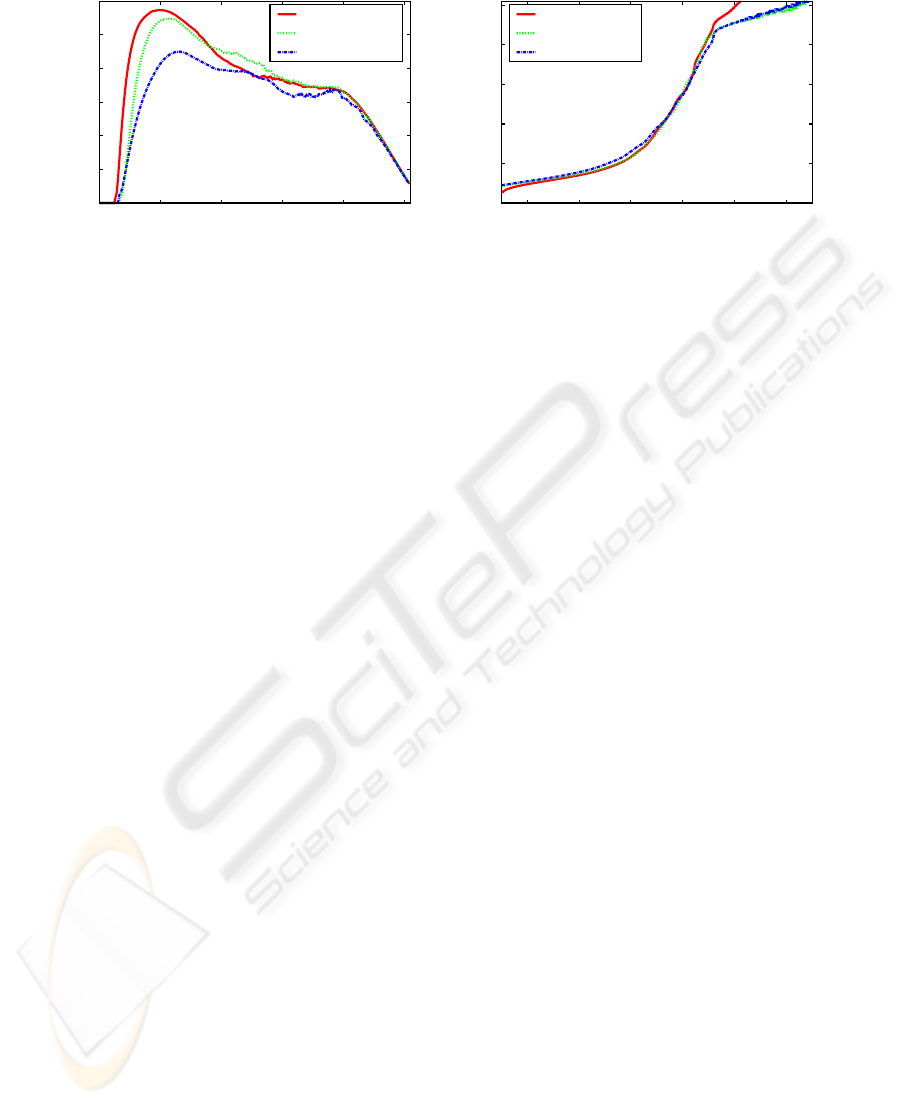
Figure 2: The curves for each color channel reconstructed independently by the proposed algorithm.
more weight to larger regions, that suggest more con-
fidence, although variances are neglected. But only
regions R of small gray value variance had been se-
lected for the computation. Fourthly, for segmenta-
tion a border around the images has been cut-off to
account for vignetting effects.
The resulting function g
′
does not produce a suffi-
ciently smooth curve, so that after computation of all
g
′
(z) with z = 0, . . . , 255 further smoothing is applied.
3.3 Recovering the Response Curve
Here a problem specific regularization term is devel-
oped, that can be used to solve equation (3). The
objective function is similar to equation (4), but the
smoothness term has been replaced by the first deriva-
tive,
O =
N
∑
i=1
P
∑
j=1
[w
z
(Z
ij
)(g(Z
ij
) − lnE
i
− ln∆t
j
)]
2
+
λ
Z
max
−1
∑
z=Z
min
+1
g
′
(z)
2
(18)
Please note, that in the regularization term the weight-
ing function w
z
has been canceled. Originally this had
been used in equation (4) to approximate the slope of
the curve g, which had been expected to be of the type
shown in figure 1. Here no assumptions are globally
made on the shape of the curve, but rather slope is es-
timated from pixel data directly, where it is locally
parametrized by equation (7). This overcomes the
restriction of the method presented in (Debevec and
Malik, 1997), that is only applicable to certain types
of sensors. Also the new regularization term is cor-
related stronger to real sensor data than the weighted
second derivative, which may be suspectible to pro-
duce results that have smoothed away valuable infor-
mation on sensor characteristics.
Debevec has proposed to choose the constant λ
so that it approximates the noise characteristics of
the sensor. Here it is not dependent on the sensor
anymore, because noise characteristics have been al-
ready incorporated by the estimated first derivative.
Although the response curve g could have been es-
timated from g
′
alone, the objective function is used
because there is varying confidence on the g
′
(z) since
some have been interpolated or at least some values
are based on a small number of data probes.
4 RESULTS AND EVALUATION
On the left, figure 3 shows four differently exposed
photographs of the set of sixteen images from the
memorial scene by (Debevec and Malik, 1997). The
images have been fused into a HDR image by the al-
gorithm presented in this paper. Firstly, the scene is
segmented by the herein proposed method over all
images at once. This produces a single segmenta-
tion result for each color channel, where the results
from the blue channel are shown in the middle-left
of figure 3. Secondly, from the segmentation about
fifty high quality regions are selected, see the middle-
right of figure 3. These are distributed evenly over
the range of gray values and spatially well, too. For
each region the location of the pixel with the lowest
edge weight is chosen as an input to the data fitting
term of equation (18). Thirdly, a set of regions with
weaker conditions is selected. From these regions of
weaker quality, with input from all images of the ex-
posure series, the first derivativeof the response curve
is estimated for every discrete gray value by equation
(14), provided that there is at least one region which
averages to the specific gray value. The amount of
regions available for any spcific gray value may vary
greatly. If no such region could have been selected
for a specific gray value, the derivative is estimated
VISAPP 2009 - International Conference on Computer Vision Theory and Applications
544
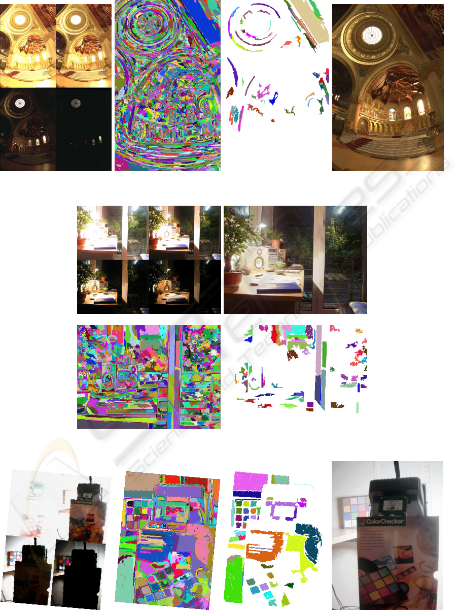
Figure 3: An exposure series, segmentation results, high quality regions only, and the downscaled HDR image.
Figure 4: Another exposure series, the tonemapped HDR image, segmentation results, and high quality regions only.
Figure 5: Yet another exposure series, segmentation results, high quality regions only, and the tonemapped HDR image.
RECOVERY OF THE RESPONSE CURVE OF A DIGITAL IMAGING PROCESS BY DATA-CENTRIC
REGULARIZATION
545

by the slope of the derivative curve itself. For this im-
age set the so computed slope is shown in figure 2 on
the left. Fourthly, from the then known slope used for
regularization and the pixel locations chosen from the
segmented high quality regions, that are for data fit-
ting, the response curve is recovered by equation (18)
and the result is shownin figure 2 on the right. Finally,
the HDR radiance map is computed by equation (5).
The result itself can not be displayed because of the
inability of display techniques to cope with the wide
dynamic range. Therefore it has been downscaled to
8-bit again and is shown in figure 3 on the right.
A second series of images provided with
(Krawczyk, 2008) is reconstructed to HDR in the
same way and results are shown in figure 4.
In figure 5 the results from another exposure se-
ries of thirteen images by (Pirinen, 2007) are provided
with a sample set of the series itself shown on the left.
Here the response is linear, and consequently its slope
is zero at every gray value. But nevertheless the same
algorithm can successfully be applied without incor-
porating any knowledge about this fact into the algo-
rithm. The final result is a tonemapped LDR image
obtained from the reconstructed HDR image and is
shown in figure 5 on the right. Here the segmentation
results are taken from the green channel.
The presented algorithm has been compared to De-
bevec’s, where the segmentation process and the se-
lection of high quality regions has been adopted to
find stable pixel locations as an input for equation
(4). Therefore both algorithms have been tested on
the same input data. It has been found that both algo-
rithms produce HDR images of comparable quality.
5 CONCLUSION
In this paper an automatic system has been presented,
that is able to fuse a series of differently exposed LDR
images into a final HDR radiance map. For this pur-
pose a linear system of equations has been used with
a here developed regularization term that is built from
original sensor characteristcs accessible by gray val-
ues of pixels. As an input trustworthy regions have
been selected by a greedily optimal segmentation al-
gorithm under the constraints of minimum variance
and maximum contrast. From the segmentation result
further regions with lower quality constraints have
been extracted and used for the computation of a data-
centric regularization term, which is the slope of the
to be estimated response curve.
Although the response curve has been recon-
structed from the knowledge of its first derivative,
which in itself had been estimated from the noisy im-
age data, the method is comparable to (Debevec and
Malik, 1997).
REFERENCES
Debevec, P. E. and Malik, J. (1997). Recovering high dy-
namic range radiance maps from photographs. In SIG-
GRAPH ’97: Proceedings of the 24th annual con-
ference on Computer graphics and interactive tech-
niques, pages 369–378, New York, NY, USA. ACM
Press/Addison-Wesley Publishing Co.
Felzenszwalb, P. F. and Huttenlocher, D. P. (2004). Efficient
Graph-Based Image Segmentation. In International
Journal of Computer Vision, volume 59, pages 167–
181. Springer.
Krawczyk, G. (2008). PFScalibration (Ver-
sion 1.4) [Computer software]. Re-
trieved August 21, 2008. Available from
http://pfstools.sourceforge.net/ and http://www.mpi-
inf.mpg.de/resources/hdr/calibration/pfs.html.
Manders, C. and Mann, S. (2006). True Images: A Calibra-
tion Technique to Reproduce Images as Recorded. In
Proc. ISM’06 Multimedia Eighth IEEE International
Symposium on, pages 712–715.
Mann, S. and Picard, R. W. (1995). Being ’undigital’ with
digital cameras: Extending Dynamic Range by Com-
bining Differently Exposed Pictures. In IS&T’s 48th
annual conference Cambridge, Massachusetts, pages
422–428. IS&T.
Mitsunaga, T. and Nayar, S. (1999). Radiometric Self Cali-
bration. In IEEE Conference on Computer Vision and
Pattern Recognition (CVPR), volume 1, pages 374–
380.
O’Malley, S. M. (2006). A Simple, Effective System for
Automated Capture of High Dynamic Range Images.
In Proc. IEEE International Conference on Computer
Vision Systems ICVS ’06, pages 15–15.
Pal, C., Szeliski, R., Uyttendaele, M., and Jojic, N. (2004).
Probability models for high dynamic range imaging.
In Proc. IEEE Computer Society Conference on Com-
puter Vision and Pattern Recognition CVPR 2004,
volume 2, pages II–173–II–180.
Pirinen, O. (2007). Image series [Computer files].
Retrieved November 17, 2008. Available from
http://www.cs.tut.fi/ hdr/index.html.
Robertson, M. A., Borman, S., and Stevenson, R. L. (2003).
Estimation-theoretic approach to dynamic range en-
hancement using multiple exposures. In Journal of
Electronic Imaging, volume 12, pages 219–228. SPIE
and IS&T.
Sprawls, P. (1993). Physical Principles of Medical Imaging.
Aspen Pub, 2nd edition.
Tsin, Y., Ramesh, V., and Kanade, T. (2001). Statistical
calibration of CCD imaging process. In Proc. Eighth
IEEE International Conference on Computer Vision
ICCV 2001, volume 1, pages 480–487.
VISAPP 2009 - International Conference on Computer Vision Theory and Applications
546
