
APPLICATION OF SCALE ANALYSIS ON LEVEL SETS FOR
COOPERATIVE IMAGE SEGMENTATION
M. Y. Benzian
1
and N. Benamrane
2
1
University of Tlemcen Algeria,
2
University of Oran, Algeria
Keywords: Segmentation, Level Sets, Curvature, Image scale.
Abstract: Image Segmentation has been used by many approaches and techniques in artificial vision but none of them
has been proved to be applied completely successfully for any image or object type. We propose in this
paper a segmentation approach based on level sets which incorporate low scale cooperative analysis of both
image and curve. The image at a low resolution level provides information on coarse variation of grey level
intensity. For the same perspective, the curve at a low resolution scale provides a coarser curvature value.
The purpose of image scale cooperative approach is to avoid stopping the curve evolution at local minima of
images. This method is tested on a sample of a 2D abdomen image, and can be applied on other image
types. The results obtained are satisfying and show good precision of the method.
1 INTRODUCTION
Image segmentation is widely used in artificial
vision. Its importance is estimated also because of its
complexity and the accuracy of results it should
provide. Explicit deformable models or active
contours were used in image processing and mostly
used in medical imaging. Explicit active contours or
snakes appeared in the paper of (Kass & al., 1988)
and (Caselles & al. 1993, 1997) gave satisfying
results especially in medical imaging but suffer from
limitations like the difficulty to track a shape of
unspecified topology. Implicit deformable models
proposed by (Osher and Sethian, 1988), and by
(Malladi & al., 1995) offer a good segmentation tool
on shapes of unspecified topology, and consequently
apply in the case of 2D medical images and can be
easily extended to 3D image volumes.
This paper treats the segmentation problem by
level sets or implicit deformable models. The model
is based on the addition of new constraints to the
speed evolution function of level curves. These
constraints are:
Local Variation of grey level intensity of a
point P in the contour. In the case of a
difference of grey level mean values between
pixels at the inside of the contour and pixels at
the outside of the contour in a local
neighbourhood of P, the function evolves at P,
else the constraint is null and the evolution
stops.
Utilization of a low level scale image and
calculation of mean grey level intensity
variation with the same manner as the first
constraint in order to eliminate local minima.
Utilization of low level scale curves computed
from the current curves in order to smooth
discrete curvatures and eliminate concavity
and convexity zones present in local minima.
In section 2 of this paper we give an outline of
implicit deformable models and level curves
evolution principle. Next, we describe in section 3 in
detail the proposed segmentation method with Level
Sets that incorporate Image and Curve analysis at
low Resolution level. In section 4, segmentation
results are shown on a 2D abdomen image. At the
end, we finish by a conclusion and future
perspectives of this work.
2 LEVEL SETS
The principle of Level Sets method is to move and
warp temporally any kind of closed curve or surface
implicitly represented (Adalsteinsson and Sethian,
1995).
224
Benzian M. and Benamrane N. (2009).
APPLICATION OF SCALE ANALYSIS ON LEVEL SETS FOR COOPERATIVE IMAGE SEGMENTATION.
In Proceedings of the Fourth International Conference on Computer Vision Theory and Applications, pages 224-230
DOI: 10.5220/0001805802240230
Copyright
c
SciTePress
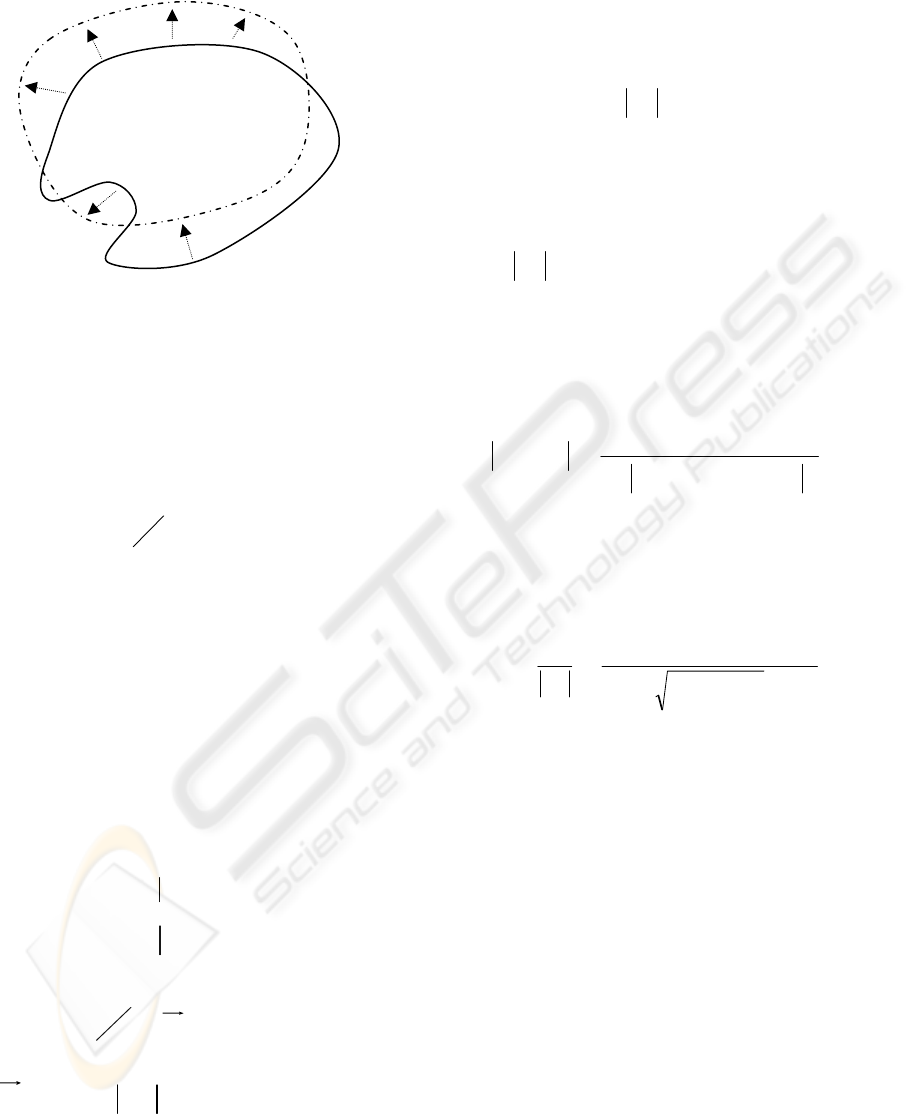
Figure 1: Evolution of a closed curve C represented by a
function Φ between time intervals t and t+∆t.
2.1 Detail of Level Sets Method
C is the level curve of the object in evolution. Φ (X,
t) < 0 inside the curve, and Φ (X, t) > 0 outside the
curve. Φ (X, t) is null on the curve C.
The closed contour C –also called front or
interface -evolves according to the equation:
NF
t
.=
∂
∂φ
(1)
F : propagation speed defined in each point of
the curve.
The level set principle is to consider the moving
curve or interface as the set of null values of a
function Φ.
We represent Φ by a 2 dimension matrix of real
numbers Φ(x,y). (x,y) are pixel coordinates on the
image. Values of Φ (x,y) that coincide with the
position of the curve C are initialized to zero. Values
of Φ (x,y) outside of the curve are positive and equal
to the euclidian distance to the curve, and the values
inside of the curve are negative.
The propagation front C is defined as:
{}
0),()( == txxC
φ
(2)
The Set
{}
0)0,()( ==txx
φ
defines
the initial contour.
Φ evolves according to the equation:
0. =∇+
φ
∂
∂φ
N
t
(3)
N : normal unit vector to the curve,
φφ
∇−∇= /N
F (curve evolution speed): it depends on external
properties, such that physical image properties like
gray level intensity, and of intrinsic properties
concerning the curve itself like the discrete
curvature.
Generally, the most used speed propagation
formula is function of image gradient g and
curvature of curve κ :
(
)
κεα
.. +∇= cIgF
(4)
This function is used for comparison in section 4
of experimental results. c : constant, generally equal
to 1. ε : term 0 < ε < 1.
α = ± 1. For α =-1, the curve expands or
increases. For α =+1, the curve shrinks.
Ig ∇ : term that computes the stopping criterion
by image gradient. It allows to minimize the distance
–variation- between the external contour and real
image borders, so that the contour of the object
coincides with the gradient of the image.
The typical formula of g (image gradient) is (p=1
or 2):
()
()
()()
p
yxIyxG
yxIg
,*,1
1
,
σ
∇+
=∇
(5)
κ : curvature that represents the viscosity term of
the speed evolution function F and improves
smoothing of the curve. The formula below shows
the relation between normal to the curve φ and
curvature κ:
()
3
22
22
2
yx
xyyxyyxyxx
div
φφ
φφφφφφφ
φ
φ
κ
+
+−
=
⎟
⎟
⎠
⎞
⎜
⎜
⎝
⎛
∇
∇
=
(6)
The function F is proportional to the curvature
and inversely proportional to the grey level intensity.
It means in general that if F(p) ≈ 0, the curve is
stable at the point p, on the other hand if abs(F(p)) >
0, the contour is instable and a curve deformation at
the point p is necessary.
The general evolution principle of « Level
Sets » or level curves (Chopp, 1993) is to calculate F
on all image positions and to evolve each time the
curve or the front at the point having the maximal
value of F. A permanent update of the value F on
each new position is computed. Since calculation on
all pixel positions is time computing expensive, the
narrow band principle developed by (Sethian, 1996 ,
1999) and (Adalsteinsson & Sethian, 1995) and
introduced initially by (Chopp, 1993) reduces
strongly time computing and limits computing of F
at pixels situated on a narrow band of width d pixels
at the inside or the outside of the evolving front. We
fixed the value of d equal to 1 in our approach.
The Fast Marching Method (FMM) is applied on
all level sets if the curve is applied on level sets
Φ (p, t)
Φ (p, t+∆t)
APPLICATION OF SCALE ANALYSIS ON LEVEL SETS FOR COOPERATIVE IMAGE SEGMENTATION
225
where the curve is always moving in the same
directions (UpWind for the expansion and
DownWind for shrinkage). The evolution to the
negative direction can be realized by inversing the
sign of the speed function.
2.2 Image Scale Analysis with Level
Sets
The Multiscale approach has been recently used with
Level Sets and Active Contour models in several
research works.
(Lin & al., 2003) apply multi-scale level set
framework to echocardiographic ultrasound image
sequences by using pyramid level resolutions. They
specify that the intensity distribution of an
ultrasound image at a very coarse scale can be
approximately modelled by Gaussian. And they
combine region homogeneity and edge features in a
level set approach to extract boundaries
automatically at this coarse scale. At finer scale
levels, these coarse boundaries are used to both
initialize boundary detection and serve as an external
constraint to guide contour evolution.
A level set approach for multiscale vessel
segmentation is proposed by (Yu & al., 2005). They
incorporate the prior knowledge about the vessel
shape into the energy function as a region
information term. Multiscale mechanism is mainly
used in vessel enhancement filtering.
(Paragios and Deriche, 2000) propose a
multiscale technique combined with level sets and
geodesic active contours. Specifically, a Gaussian
pyramid of images is built upon the full resolution
image and similar geodesic contour problems are
defined across the different levels. The
multiresolution structure is then utilized according to
a coarse-to-fine strategy, an extrapolation of the
current contour from a level with low resolution to
levels with finer contour configuration takes place.
They apply their method to a pyramid with 2 or 3
levels of resolution. The
multiscale approach
especially permits moving objects to be tracked with
considerable speedup.
In the next section, we propose our method that
computes and analyses both image and level set
curve at lower scale level.
3 COOPERATIVE IMAGE SCALE
ANALYSIS WITH LEVEL SETS
We have adopted a new segmentation approach with
level sets by the integration of a Multi-scale
approach. The classical formula of F (4) has been
modified by a new one in order to improve avoiding
local minimum. In our work, we have used
Multiscale for image intensity and curve
computation at lower resolution level. The lower
scale image and curve enable respectively to
calculate local image intensity variation and discrete
curvature value at a coarse level.
3.1 Local Gray Level Constraint
This new constraint is added to the speed function F.
We consider a local rectangular zone F with size
(m x m) at the neighbourhood of the point P.
Generally, the evolution of a contour at a given point
P can affect the evolution of the close pixels with P
in the same direction.
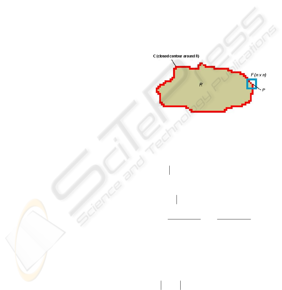
Figure 2: Local Window (n x n) for computing the local
gray level variation in the image.
The neighbourhood zone F is centered at the
point
ij
P with radius n. The radius value used here is
2.
{
}
njynjnixnixF +≤≤−+≤≤−= ,
(7)
The actual interface or Contour C delimits the
region R (Fig. 3).
{
}
121
,; EFEFxRxxE −=∈∈=
(8)
(
)
()
()
()
2
2
2
1
1
1
,
ECard
Exi
l
ECard
Exi
l
∑
∑
∈
=
∈
=
(9)
l
1
(resp. l
2
): mean grey level pixels of the set E
1
(resp. E
2
).
1
l : mean grey level of pixels inside the window
F and belonging inside the region R delimited by the
contour C. i(x): image intensity of a pixel in the
window F.
If
⇒≈− 0
21
ll there is no local grey level
variation at the point P, then the level curve C must
evolve at P.
VISAPP 2009 - International Conference on Computer Vision Theory and Applications
226
If
⇒>− 0
21
ll there is local gray level
variation at the point P.
The local mean gray level formula is:
()
k
loc
ll
MG
21
1
1 −+
=
ν
(10)
ν
1
is a weighting coefficient, k = 1.
3.2 Lower Scale Image and Curve
computation
3.2.1 Lower Scale Image Computation
To compute a lower scale resolution image, we
apply Bartlett filter to the image, by reducing with a
scale value of four (4).
The mask (3 x 3) of the Bartlett filter below
is applied to derive a lower scale image by a value of
2 after a Gaussian smoothing of the image. In the
case of computing an image with a lower scale value
of 4, we apply to the image a composition operation
of Bartlett filter 2 times successively.
[]
121
4
1
.
1
2
1
4
1
121
242
121
16
1
33
⎥
⎥
⎥
⎦
⎤
⎢
⎢
⎢
⎣
⎡
=
⎥
⎥
⎥
⎦
⎤
⎢
⎢
⎢
⎣
⎡
=
def
x
bartlett
h
The figure (3) shows the original image and the
image obtained by division with a scale factor of 4,
by a successive reduction for 2 times with a scale
factor of 2. Section 3.3 will give more details about
this constraint.
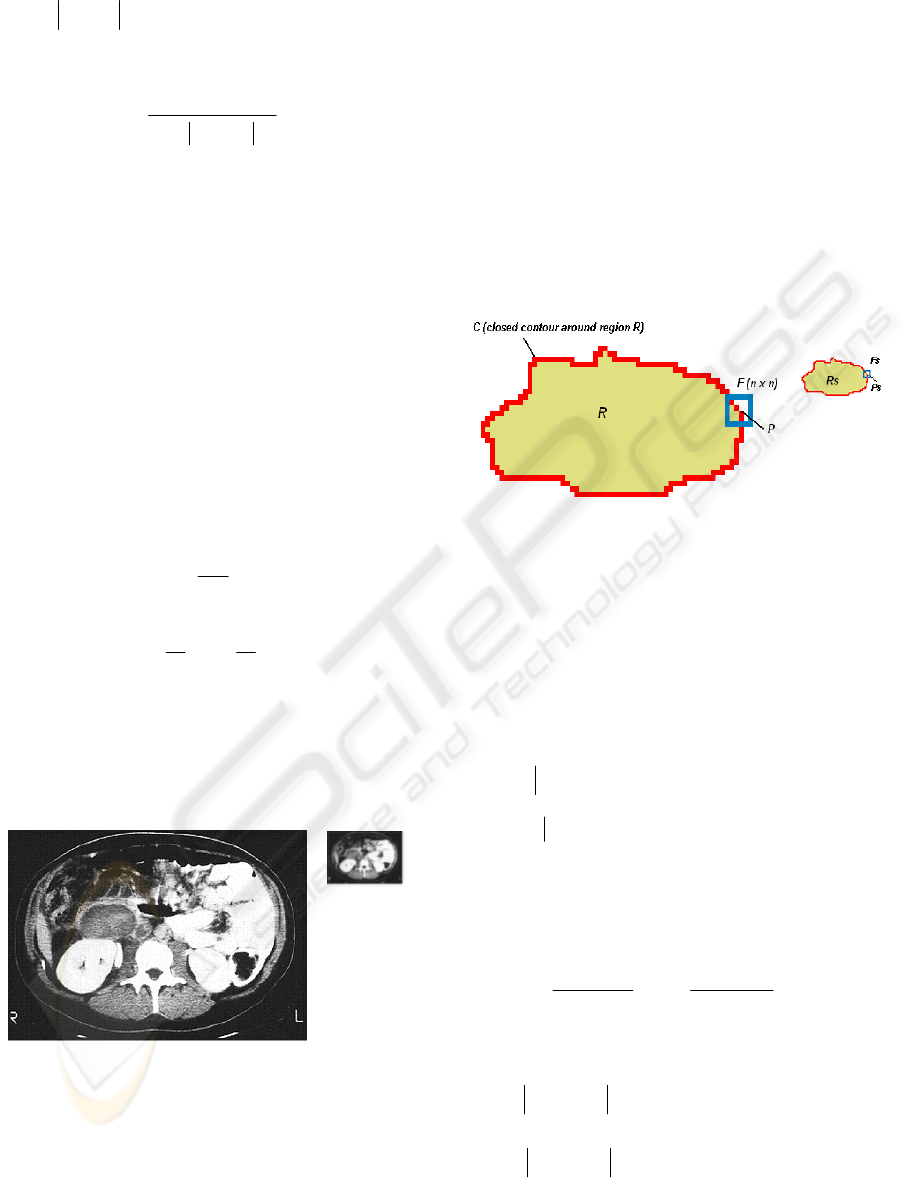
Figure 3: Original Image and image I
S
with a scale factor
of ¼.
3.2.2 Lower Scale Curve Approximation
The computation of a curve at a lower scale and
corresponding to the original curve is generated
approximately.
The original closed curve represents a Narrow
Band of a zero level set of width 1 that delimits the
deforming object in segmentation. Pixels P (x, y) of
the closed curve are represented by a list L of points.
The computation of a curve at a low scale is
realized by dividing each pixel position (x, y) of L
by the same scale value applied to the image. We
obtain a new list L
S
of points (x
S
, y
S
), redundant
pixel values of (x
S
, y
S
) are automatically eliminated.
Figure 4 shows the region R
S
delimited by the
low scale Curve Ф
S
after image reduction by a scale
factor of 4. Section 3.4 will give details about the
application of this constraint.
Figure 4: The region R
S
is derived from region R after
scale factor applying in the image.
3.3 Local Gray Level Variation
Constraint in Lower Scale Image
The neighbourhood zone F
S
of the scaled image is
centered at the point P
S
ij
with radius n. The radius
value used here is 2.
{
}
njynjnixnixF
S
+≤≤−+≤≤−= ,
(11)
{
}
121
,; SFSFxRxxS
SSS
−=∈∈=
(12)
Sl
1
: mean grey level of pixels of the local zone
F
S
and belonging inside of the region R
S
delimited
by the low scale Curve Ф
S
after image reduction by
a scale factor s.
() ()
2
2
2
1
1
1
,
SCard
Sx
sl
SCard
Sx
sl
∑
∑
∈
=
∈
=
(13)
Sl
1
(resp. Sl
2
): mean grey level pixels of the set
E
1
(resp. E
2
).
If
⇒≈− 0
21
slsl the curve must evolve,
there is no intensity variation in the image.
If
⇒>− 0
21
slsl there is a local coarse
intensity variation.
APPLICATION OF SCALE ANALYSIS ON LEVEL SETS FOR COOPERATIVE IMAGE SEGMENTATION
227
()
k
loc
slsl
ScaleMG
21
2
1
_
−+
=
ν
(14)
ν
2
is a weighting coefficient, k = 1.
Example: figure 5 presents 2 images with an
initial contour (yellow) in the left image and a final
contour (full red) in the right image, and where the
final contour cannot segment and add the local grey
level variation inside the contour by using simply
the classical level set evolution function
Figure 5: Image Segmentation Result by classical Level
Sets method.
3.4 Lower Scale Discrete Curvature
Constraint
This constraint is based on the computation of the
geometrical shape contour at a lower scale to obtain
a coarser contour, then the computation of the
discrete curvature value at a point P
S
of the lower
curve (fig. 6B), in order to eliminate coarser concave
or convex shapes that are also smoothed.
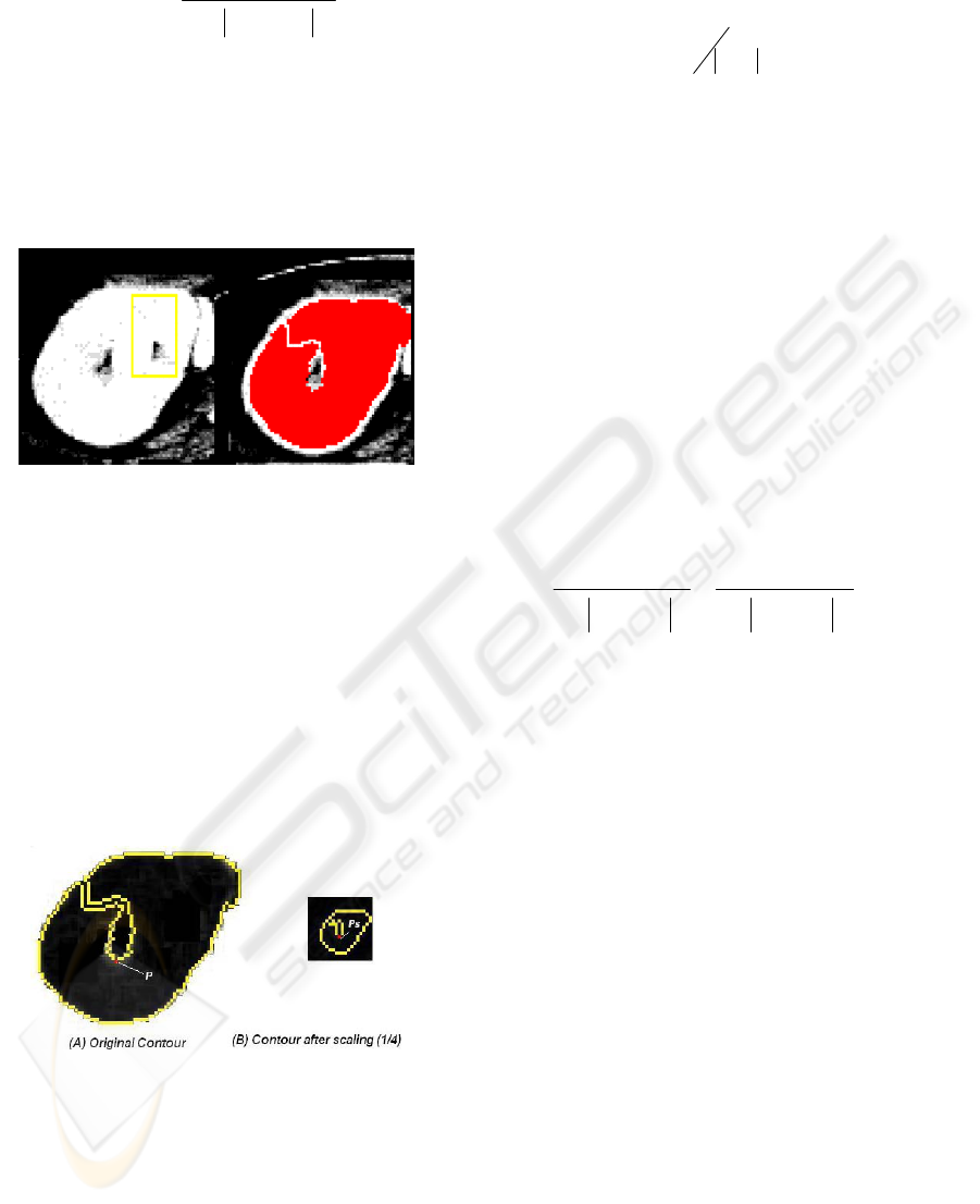
The figure 6 shows an example of the contour
and its scaling by a factor of 4.
Figure 6: Original Contour (A) and the generated Contour
(B) after scaling, the point P
S
(red) after scaling
corresponds to the point P (red) of the original contour, so
the point P
S
corresponds to more than one point P (approx.
4 points for a scale value of 4) of the original contour.
κ
s
: discrete curvature: the curvature formula is
the same as the formula (6) applied for the curvature
κ, after applying a transformation –reduction with a
scale 1/s- to the original contour in order to smooth
contour positions that still present convex or
concave parts at a large scale.
⎟
⎠
⎞
⎜
⎝
⎛
∇
∇
=
S
S
S
div
φ
φ
κ
(15)
This method estimates the curvature value at a
lower resolution level. Ф
S
: curve of the right image
(fig 6.B) obtained at a lower resolution level.
3.5 Speed Function F or Level Set
Evolution Function
The precedent constraints (sections 3.1 to 3.4) are
integrated to the speed evolution function F. The
value of F is computed at each point of the curve C.
The formula of F is as follows by integrating
formulas (10) and (14) for local gray level constraint
and local gray level at lower scale constraint
respectively :
(
)
S
gF
κ
α
κ
α
..
2
+
±
=
(16)
locloc
ScaleMGMGg _
+
=
(17)
21
21
2
21
1
11
kk
slslmm
g
−+
+
−+
=
ν
ν
(18)
g: image intensity variation. k
1
, k
2
= 1.
κ : discrete curvature for curve smoothing.
κ
S
: discrete curvature of the scaled curve (this
value is coarser and is computed only for points
whose curvature value κ is not high).
ν
1
, ν
2
: weighting coefficients. α, α
2
: weighting
coefficients, generally lower than intensity
coefficients ν
1
, ν
2
.
The coefficient values are determined
empirically and experimentally.
The sign of F indicates the evolution direction of
the curve. In the case of this approach, the direction
is manually chosen by the user, and by default
negative, which means that the initial curve is in
expansion or dilation, and hence limits the evolution
to Fast Marching where the curve evolves only in
one direction, UpWind or DownWind.
If F < 0 → the contour expands and the front
evolves only at the outside of the curve.
If F > 0 → the contour shrinks and the front
evolves only at the inside of the curve.
If F ≈ 0 → the contour is stable.
What position P of the curve to choose for
moving the front? Select the pixel or the position
having the absolute value of F maximal.
VISAPP 2009 - International Conference on Computer Vision Theory and Applications
228
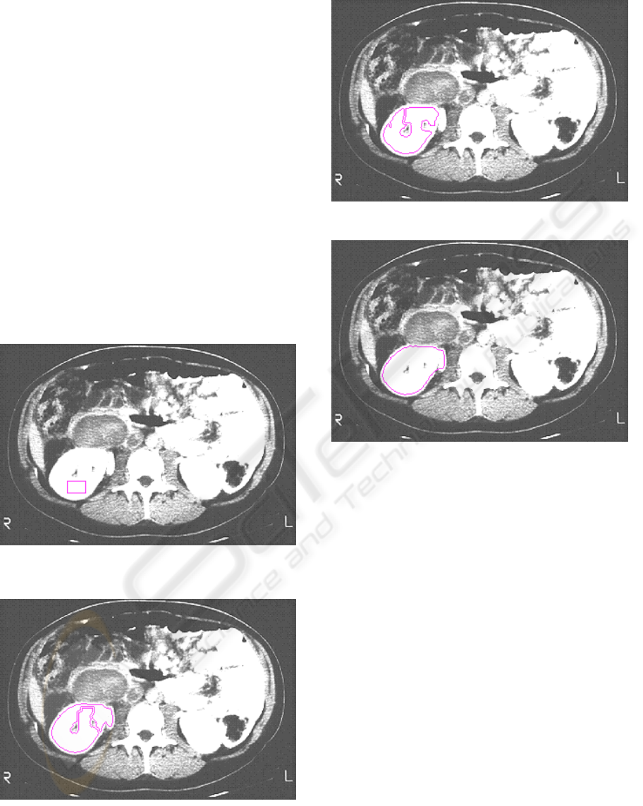
4 EXPERIMENTAL RESULTS
We applied our approach to a 2D abdomen image.
Figure 7 shows the original image with the initial
contour.
Figure 8 shows the result of the segmentation
with the classical level set function by applying the
formula (4) of the propagation speed related in
section 2. The 2 local minima inside the object are
not segmented.
Figure 9 shows a partial result of the
segmentation progression by integrating the
constraints of our approach described in section 3.
Weighting coefficient values for grey level
variation ν
1
and ν
2
are equal to 2 and 1 respectively.
The value of coefficient α used is 0.20. The
value of α
2
is 0.20 too if the curvature value κ is
weak (κ < κ
max
/2); else α
2
= 0 is not used.
In Figure 10, the final segmentation result is
presented. The contour does not stop at the 2 local
grey level minima inside the object to be segmented.
Figure 7: Abdomen Image. Contour Initialisation by a red
rectangular zone.
Figure 8: Segmentation by traditional Levels Sets
function.
Figure 9: Partial Segmentation Result.
Figure 10: Final Segmentation Result.
5 CONCLUSIONS
In this paper, we proposed a new image
segmentation method applied with the level set
approach. Zero Level Sets or Level Curves are an
efficient tool to segment objects with unspecified
topological shape. They are depending essentially on
edge gradient for image stopping criterion and on
curvature for curve smoothing. However, stopping
the curve at a local minimum cannot be resolved
only with image gradient and discrete curvature. In
our approach, we added three constraints: (i) local
image intensity variation criterion, (ii) image
intensity variation at a lower scale and (iii) discrete
curvatures of the original curve and of the curve
obtained at a lower scale in order to avoid stopping
the curve at local grey level minima of the images.
We hope to extend our segmentation approach to
different image types and to 3D image volumes.
APPLICATION OF SCALE ANALYSIS ON LEVEL SETS FOR COOPERATIVE IMAGE SEGMENTATION
229

REFERENCES
Adalsteinsson, D., Sethian, J.A., 1995. A Fast Level Set
Method for Propagating Interfaces. In Journal
Computational Physics, 118, 2, pp. 269-277.
Baillard, C, Barillot, C, Bouthemy, P, 2000. Robust
Adaptive Segmentation of 3D Medical Images with
Level Sets. INRIA, Research Report, Rennes, France,
Nov. 2000
Caselles, V, Katte, F, Coll T, Dibos, F, 1993. A geometric
model for active contours. Numerische Mathematik,
vol. 66, pp 1-31.
Caselles, V, Kimmel, R, Sapiro, G, 1997. Geodesic active
contours. International Journal of Computer Vision.
Chopp, D. L, 1993. Computing Minimal Surfaces via
Level Set Curvature Flow. In Journal Of Comp. Phys.,
vol 106, pp 77-91.
Kass, M, Witkin, A, Terzopoulos, D, 1988. Snakes: Active
contour models. Int J. Comput. Vis., vol. 1, pp 321-
331.
Lin, N, Yu, W, Duncan J.S., 2003. Combinative multi-
scale level set framework for echocardiographic image
segmentation. Elsevier, Medical Image Analysis, vol.
7, pp 529-537.
Malladi, R, Sethian, J.A., Vemuri, B.C. 1995. Shape
modeling with front propagation : a level set approach.
IEEE Transactions on Pattern Analysis and Machine
Intelligence, vol. 17, pp 158-175.
Osher, S, Sethian, J.A., 1988. Fronts Propagating with
Curvature-Dependent Speed : Algorithms Based on
Hamilton-Jacobi Formulations. In Journal of Comput.
Phys.
Paragios, N., Deriche, R. 2000. Geodesic active contours
and Level sets for the detection and tracking of
moving objects. IEEE Transactions on Pattern
Analysis and Machine Intelligence, vol. 22, nr 3, pp
266-280.
Sethian, JA, 1999. Level set methods and fast marching
methods: Evolving interfaces in computational
geometry, fluid mechanics, computer vision, and
material science.
Sethian, J.A., 1996. A Fast Marching Level Set Method
for Monotonically Advancing Fronts. Proc. Nat. Acad.
Sci., 93, 4, pp.1591--1595.
Yu, G, Miao, Y, Li, P, Bian, Z, 2005. Multiscale vessel
segmentation: a Level set approach. 10th
Iberoamerican Congress on Pattern Recognition,
CIARP. Havana, Cuba, November 15-18, pp 701-709.
VISAPP 2009 - International Conference on Computer Vision Theory and Applications
230
