
SELF-CALIBRATION CONSTRAINTS ON EUCLIDEAN
BUNDLE ADJUSTMENT PARAMETERIZATION
Application to the 2 Views Case
Guillaume Gelabert, Michel Devy and Frédéric Lerasle
CNRS; LAAS; 7 avenue du Colonel Roche, 31077, Toulouse, France
Université de Toulouse; UPS, INSA, INPT, ISAE; LAAS; Toulouse, France
Keywords: Self-calibration, Focal estimation, 3D reconstruction, Bundle adjustment.
Abstract: During the two last decades, many contributions have been proposed on 3D reconstruction from image
sequences. Nevertheless few practical applications exist, especially using vision. We are concerned by the
analysis of image sequences acquired during crash tests. In such tests, it is required to extract 3D
measurements about motions of objects, generally identified by specific markings. With numerical
cameras, it is quite simple to acquire video sequences, but it is very difficult to obtain from operators in
charge of these acquisitions, the camera parameters and their relative positions when using a multicamera
system. In this paper, we are interested on the simplest situation: two cameras observing the motion of an
object of interest: the challenge consists in reconstructing the 3D model of this object, estimating in the
same time, the intrinsic and extrinsic parameters of these cameras. So this paper copes with 3D Euclidean
reconstruction with uncalibrated cameras: we recall some theoretical results in order to evaluate what are the
possible estimations when using only two images acquired by two distinct perspective cameras. Typically it
will be the two first images of our sequences. It is presented several contributions of the state of the art on
these topics, and then results obtained from synthetic data, so that we could state on advantages and
drawbacks of several parameter estimation strategies, based on the Sparse Bundle Adjustment and on the
Levenberg-Marquardt optimization function.
1 INTRODUCTION
This paper proposes some simple comparative
results concerning the precision of the absolute 3D
Euclidean reconstruction we can expected from 2
different pinholes cameras and from matched points
between views. The cameras are supposed to have
very distinct relative orientations, so that it cannot be
considered as a stereovision head; cameras
parameters are unknown, except focal lengths that
are approximately known from the constructor’s
data sheet. We focus on the projective reconstruction
of 3D points from matched pixels on two views and
on the quality of the Euclidean structure estimated
without prior geometric information, but imposing
constraints/priors on the cameras parameters space.
Imposing priors on the parameters may give better
theoretical precision rather than fixing parameters.
Nevertheless one must take care about
parameterization imposed by the self-calibration
constraints. We will particularly insist on this point.
This work is motivated by an application about the
analysis of video sequences acquired by two or more
cameras, typically on a crash test experiments. Two
images are presented on Figure 1: they are acquired
by two uncalibrated cameras with very different
viewpoints. The challenge consists in extracting 3D
information from these images recovering in the
same estimation process, the intrinsic parameters of
the two cameras.
2 CAMERA MODEL
We are looking for the best Euclidean 3D
reconstruction we can obtain from m sets of n
corresponding images points x
ij
coming from n 3D
point X
i
, projected onto the image planes by m
distinct pinhole cameras P
j
. To reach this goal, we
want to estimate a parameter vector p that contain
the camera parameters (P
j
projection matrix for the
camera j) and the 3D points
573
Gelabert G., Devy M. and Lerasle F. (2009).
SELF-CALIBRATION CONSTRAINTS ON EUCLIDEAN BUNDLE ADJUSTMENT PARAMETERIZATION - Application to the 2 Views Case.
In Proceedings of the Fourth International Conference on Computer Vision Theory and Applications, pages 573-579
DOI: 10.5220/0001806205730579
Copyright
c
SciTePress

p = (P
j
, X
i
)
(1)
Without considering optical distortions, we have a
total of (11m+3n) parameters. The parameter vector
p gives a predictive camera model
u
ij
: R
11
x R
3
→R
2
(2)
The model is for the 3D point i seen by the camera j:
ij ij ij j i
x = u (p) = P X i=1...n, j=1...m
λ
(3)
The model will impose implicit constraints,
c(x
ij
, u
ij
) = 0 (4)
between underlying feature x
ij
from noisy measurements
of the feature x’
ij
, and have to be consistent with the
feature.
2.0.1 Feature Error Model
Due to the very distinct viewpoints of the cameras,
the feature points are selected manually and suppose
free from outliers. The observation noise d(x
ij
)
induced by this manual selection is assumed to have
Gaussian independent and identically distributed
terms, with variance s
2
.
x’
ij
= x
ij
+ d(x
ij
)
(5)
2.0.2 Cost Function
We have chosen the Maximum Likelihood Estimator
(MLE) as decision criterion to estimate the
parameters that best fit to the feature error model.
MLE gives the global minimum of the inverted log
likelihood, taken as a function of the parameters p,
p
p = argmin J(p)
(6)
With
()
2
n,m
2
ij ij
i,j=1
1
J(p) = x -u p
2σ
∑
(7)
It is well known that this cost function does
generally not have a unique minimum and is very
dependent on the initial estimate of the parameters
p
0
. These problems occur if it exists a coordinate
transformation g of the parameter space P such that
J(p) = J(g.p)
(8)
The set of all such transformation form the group G,
called the group of gauge transformation. The set of
all parameters such that p = g.p
0
(p is geometrically
equivalent to p
0
) form what is called the leaf Pp
0
associated with p
0
, which is a sub manifold of P. So
some constraints have to be imposed on the
parameters set in order to have a unique solution,
which minimizes eq.(7), for each connected
component of the leaf. However we recall that this
will not be a global minimum of J. Moreover, these
constraints need to be linear.
2.0.3 Numerical Optimization
The Non Linear Least Square problem defined by
MLE eq.(7) will be solved by numerical
optimization via a Damped Levenberg-Marquardt
algorithm allowing simple bounds constraints on the
variables (Gill et al., 1981) , also called a Bundle
Adjustment procedure (Triggs et al., 2000) as the 3D
point coordinates are part of the parameters vector p.
2.1 Counting Argument
If we consider that the m cameras are uncalibrated,
the projection matrixes P
j
contain 11m independent
parameters, removing the projective scale factor.
These parameters are only defined up to 15 degrees
of freedom (noted dof) coordinates transformation T
of the projective space P
3
, defining a camera
parameter space with (11m-15) essential degrees of
freedom (noted edof).
That simply means that to have a unique solution on
the leaf Pp
0
, the parameters must be constrained by
15 algebraically independent gauge equations c
i
.
These equations define a sub manifold C in P of co
dimension 15 and ensure that there is a unique gauge
transformation g that maps a parameter p of Pp
0
to
another parameter pc of Pp
0
which respects the
constraints.
Now, let us consider the same problem with
calibrated cameras: every projection matrix has 6
dof, and are defined only up to a 7 dof similarity
transformation of the Euclidean coordinate space,
leaving (6m-7) edof for the parameter space. So
intuitively, if we want to move from the uncalibrated
projective space to the calibrated Euclidean space or
goes in the inverse way, we have (5m-8) edof left
and 8 constraints more to impose.
2.2 Parameterization
The classical way of representing a perspective
camera is to define the following model for a camera
projection matrix
P
j
= K
j
E
i
(10)
1
ij ij j i
x = (P T)(T X ) i=1...n, j=1...m
λ
−
(9)
VISAPP 2009 - International Conference on Computer Vision Theory and Applications
574
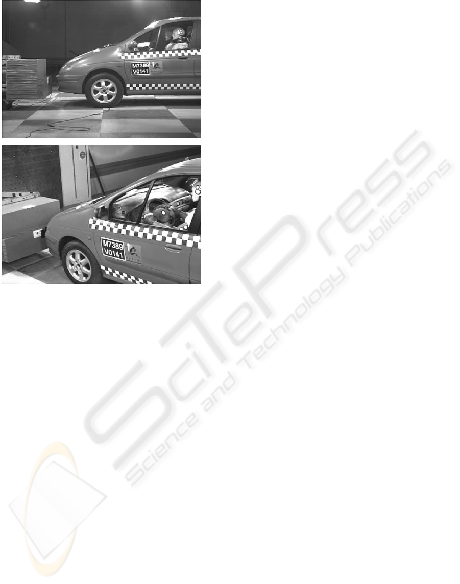
Figure 1: Example of a two-cameras application.
where K
i
is the 3X3 upper triangular intrinsic matrix (5
dof) that links 3D point coordinates in the camera
reference frame to images 2D pixel coordinates,
iu i0
iv i0
fsu
K= 0 f v
001
i
i
⎡⎤
⎢⎥
⎢⎥
⎢⎥
⎣⎦
(11)
E
i
is the extrinsic parameters matrix (6m dof), that
links the world coordinates to the cameras ones.
E
i
= [ R
i
| t
i
] (12)
However, this model will impose non linear constraints on
the feature instead of linear ones.
2.2.1 Calibrated Case
In the calibrated case, intrinsic parameters are
known, leaving a (6m) dof parameterization. So,
beginning from an initial parameter vector p
0
, 7
independent constraints have to be imposed on the
camera parameters space to have a unique solution
among C. Indeed without gauge, Euclidean
reconstruction is obtained up to a similarity. A
solution is to fix arbitrarily the world coordinate
frame to the first camera frame by imposing that
E
1
= [I
3X3
|0] (13)
and to fix the unknown scale of the Euclidean
reconstruction (Kanatani and Morris, 2000,
Grossman and Victor, 1998) by imposing
|| t
2
….t
m
|| = 1 (14)
This is the standard Euclidean gauge. We then
parameterize minimally the cameras relative
orientations by 6*m-7 free parameters, independent
from each other’s: 3(m-1) Euler angles via the
Rodrigues formula and (3m-4) parameters for the
normalized multi-camera translation. The
constrained parameter space C has (6m-7) edof.
2.2.2 From Calibrated Euclidean Space to
Uncalibrated Projective Space
Now, if we want to extent the calibrated Euclidean
parameterization defined above to the particular case
of uncalibrated cameras, the intrinsic parameters of
m cameras must be added into the system
parameterization. Beginning with totally unknown
intrinsic parameters, the projective cameras are
parameterized in a calibrated Euclidean way. The
counting argument allows (5m-8) edof to
parameterize the intrinsic parameters considering the
simple difference between the edof in the Projective
and Euclidean cases; equivalently it makes
mandatory to have 8 constraints on the (5m) dof of
free intrinsic parameters. If we denote f the fixed
intrinsic parameters and k the known ones among
the m views, we can derive the well known counting
process
mk+(m-1)f = 8 (15)
By the way, we recover the “self-calibration”
constraints, which explain the fact that “the intrinsic
parameters should be parameterized so that the self-
calibration constraints are satisfied” (Pollefeys at al.,
1998).
The Euclidean uncalibrated parameterization impose
implicit constraints on the projective parameter
space via
K [R | t] = P T (16)
which is directly related with the constraint
described by Triggs (Triggs, 1997)
P Q PT = KK
T
(17)
This constraint is applied on the absolute quadric
and is expressed algebraically by the above counting
argument.
Q = T Diag(1,1,1,0) T
T
(18)
SELF-CALIBRATION CONSTRAINTS ON EUCLIDEAN BUNDLE ADJUSTMENT PARAMETERIZATION -
Application to the 2 Views Case
575

We can visualize these 8 constraints, fixing the
unknown projective scale, by taking
P
proj
= [I
3X3
|0] (19)
so that T and so Q, are parameterized by 8
parameters (5 for intrinsic/absolute conic parameters
and 3 for the plane at infinity). It gives a local
parameterization of our gauge group G (Triggs,
1998).
T
K0
T=
p
1
⎡⎤
⎢⎥
⎣⎦
(20)
We have now (11m-15) dof for our set of
parameters; it is consistent both with the number of
edof of the projective space and with the counting
argument rule to well parameterize the intrinsic
parameters following the number of views and the
priors we have about them. It is also important to
mention that the counting argument is only valid for
non-critical configurations (configurations that do
not permit to locate exactly the absolute quadric in
the projective space). These configurations depend
either on 3D points parameters (critical surface
(Hartley and Zisserman, 2006)), or relative positions
between cameras (critical motion sequences as
described by Sturm (1997)), or both of them. Some
specific approaches have to be developed in such
cases.
2.3 Dealing with Parameters Inter
Correlations
However, using this natural approach, we are not
able to ensure that our essential parameters defined a
set of independent parameters. The calibrated
Euclidean parameterization provides an independent
set of parameters, but in the uncalibrated case, the
chosen parameterization gives intercorrelations, as
the intrinsic parameters are highly correlated with
the extrinsic ones (Shih et al., 1996). For instance,
the principal point position is correlated with the
camera orientation and the focal length with the
translation along the optical axis. In this case, the
camera parameters covariance matrix contains some
abnormally elevated values. As a consequence,
intrinsic gauge constraints imposed by eq.(10), if
perturbed by noisy measurements, will greatly
impact the Bundle Adjustment as the free parameters
will move to compensate this initial error induced by
the badly fixed/known ones.
So we could think that a free intrinsic gauge
approach, like the one proposed by Malis and Bartoli
(Malis and Bartoli, 2001) will greatly improve the
solution. Basically, the authors adopt an elegant
method, equivalent to obtain a reduced model of the
parameter set by the classical way. If we
differentiate eq. (7) with respect to the intrinsic
parameters, we set the result to zero, and we solve
the resulting equation, then, intrinsic parameters are
expressed in terms of the remaining parameters
(image point, extrinsic and 3D points). Substituting
it into eq. (3) we will obtain a function of the
remaining parameters. However, as the intrinsic
values are embedded in the free intrinsic gauge
parameterization, the self-calibration constraints still
have to be needed on remaining parameters leading
to the same problem; they are imposed either by
Lagrange multipliers or weighting methods.
A method to have a better Euclidean reconstruction
is to use some priors about the free parameters
during the optimisation, imposing the free
parameters to stay between some bounds. In the next
section, we propose some comparative results using
priors on focal lengths during a Bundle Adjustment
process, in the typical standard Euclidean gauge
(process noted EBA hereafter). For the 2 view case
with distinct cameras, EBA process is applied with
a weighting method, with bounds constraints, and
using Malis and Bartoli intrinsic free
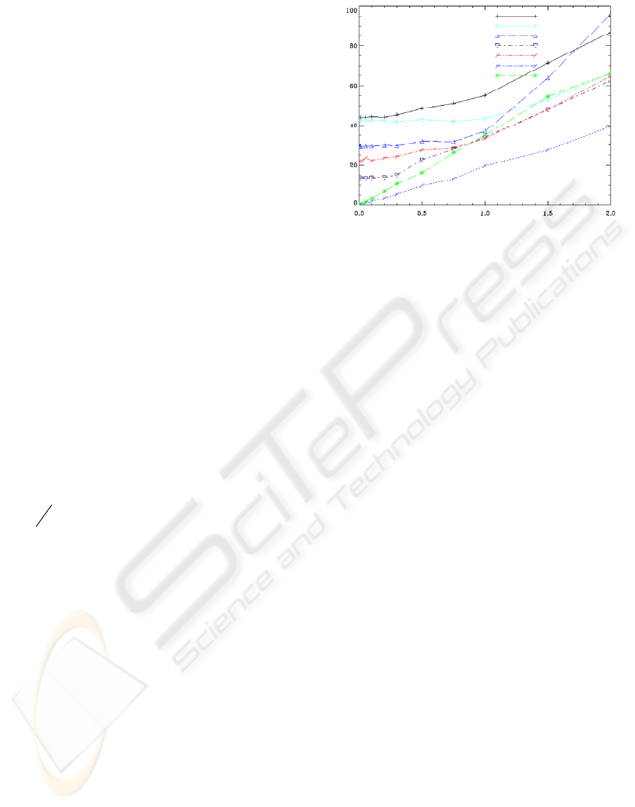
parameterization with artificial weights. Results can
be found on Figure 2.
3 TWO VIEWS CASE
Our objective here consists in comparing several
ways to calibrate a two-cameras system, depending
on initial knowledge available on the intrinsic
parameters. Seven algorithms are compared.
3.1 Parameter Choice
The number of projective edof authorizes us to
parameterize the space parameters with 7 parameters
that must ideally be independent, being far from the
possible critical configurations for self-calibration
and 3D reconstruction: a theoretical study for these
ones has been performed by Sturm (Sturm, 1997) for
the specific two view case. We recover by the way,
the 7 dof of the fundamental matrix (scaled matrix of
rank 2), which encapsulates the 2 views epipolar
geometry. This is a classical way to show that 2
camera intrinsic parameters can be recovered from
images alone by a self-calibration procedure, as it
has been shown in a pioneered contribution by
Hartley for the focal length in 1993(Hartley and
Zisserman, 2006).
VISAPP 2009 - International Conference on Computer Vision Theory and Applications
576

Using the above Euclidean camera model with the
Euclidean standard gauge, we can add to our 5
Euclidean parameters space, 2 more parameters
chosen among the intrinsic ones to reach the 7
parameters allowed. If we add more parameters, we
will neither obtain a good 3D reconstruction nor
good estimate of the intrinsic parameters
(Bougnoux, 1998, Grossman and Victor, 1998) as
the parameterization will not respect the self-
calibration constraints and will be over-
parameterized.
Let us define two situations: (1) we can suppose that
we have estimated the camera calibration parameters
by some way, e.g. reading the camera data sheet: we
know approximately the focal lengths, and can make
the usual square pixel assumption (s=0, fu = fv = f)
with (u0, v0) at image centres. (2) Using a
calibration pattern, we can also consider focal
lengths as unknown parameters and fix the other
ones to their initial values. So that our set of
parameters p = (pC, pX) are the camera parameters
pC = (f1, f2, rx, ry, rz, tx, ty) plus the unknown 3D
points pX = (X1…XN), with the standard Euclidean
gauge and the self-calibration constraint imposed by
fixing all the intrinsic parameters apart from the 2
distinct focal lengths.
3.2 Initialisation
First we recover the relative camera orientation with
the Essential matrix, via the estimated intrinsic
parameters and the fundamental matrix calculated
with the Gold Standard Algorithm (projective BA)
as described in (Hartley and Zisserman, 2006).
The initial Euclidean reconstruction of the 3D points
is obtained with the 2 view optimal methods as
described in (Hartley and Zisserman, 2006).
If the true intrinsic are used, we call the obtained
reconstruction, the
initial calibrated reconstruction,
and the
initial pre-calibrated one if initial
parameters are only approximated. This provides
two initial parameters set (p
01
, p
02
) used as initial
guesses for the Bundle Adjustment function.
3.3 Algorithms
We recall that the goal is not to recover very precise
focal lengths, but to allow a better reconstruction of
the scene by adding the 2 focal lengths as parameters
during the optimisation process.
First of all, we run the optimization (BA) with the
standard Euclidean gauge for the initial calibrated
reconstruction and initial calibrated one. Only
Extrinsic and 3D points are free during the
optimisation process. We obtain respectively the
reconstruction called
EBA calibrated and EBA
pre-calibrated
. The first one being the best 3D
reconstruction we can obtain from noisy
measurements without constraint on the structure
parameters. These will be our reference data, as the
algorithms used to obtain it are well known.
Then, even if results do not appear here, we have
verified that if there is only noise on the focal
lengths, the free 7 parameters, exactly converge
through the exact focal lengths values. This means
that self-calibration constraint and Euclidean gauge
defined a unique minimum on the parameter set, and
not a sub manifold of the parameters set. This result
is also true for more cameras as long as the camera
parameterization and the Euclidean gauge impose 15
independent gauge constraints, which can easily, be
verified experimentally.
Next we investigate the results of our algorithms,
when the self-calibration constraints are badly
defined by coarse approximations of the intrinsic
parameters, so that the correlation between intrinsic
and extrinsic parameters (Shih et al., 1996) leads to a
set of parameters that have not the required edof.
To control the focal lengths during the BA process,
it is assumed that we have probabilistic priors f =
N(f
0
, s
f
) about them. A study of the focal length
variability versus optical centre can be found in
(Willson and Shafer, 1993).
In the intrinsic free Euclidean BA called
EBA
intrinsic free, these priors are added by imposing a
weight value to the cost function of the form ||f-f
0
||
sf
where the focal is a function of remaining
parameters; other constraints coming from the fixed
intrinsic parameters are imposed by adding heavily
weighted artificial measurements as their variances
are supposed to be null.
The same procedure applied to the pre-calibrated
case, leads to the reconstruction called
EBA pre-
calibrated weighted
reconstruction.
We use then the numerical optimisation described in
(section 2.2.3) where focal lengths are subject to
linear bounds constraints (Gill et al., 1981) during
the non linear least square optimisation eq.(21),
leading to the
EBA pre-calibrated bounds
reconstruction.
0j j
7+3M
p= R
i=1..M
j=1,2
min J(p) subject to |f -f | 2
∈
≤
(21)
3.4 Synthetic Image Data
We model the object scene by 20 points randomly
created in a sphere of diameter 1000 of centre (0, 0,
SELF-CALIBRATION CONSTRAINTS ON EUCLIDEAN BUNDLE ADJUSTMENT PARAMETERIZATION -
Application to the 2 Views Case
577
0). The 20 points agree with the maximum pair of
points an operator can reasonably pick up in images
pair.
The two modelled cameras are of respective centres
C1(1866, 316, 3523) and C2(-3922, 358, 6963) with
2 respective optical axis pointing towards two
distinct points of the scene Z1(-0.35, -0.15, -0.92)
and Z2(0.51, -0.04, -0.85). The Y axis of each
camera is nearly parallel to the ground, in order to
model a realistic situation not critical for the self-
calibration of the 2 distinct focal lengths (Sturm,
1997). Ground truth is given by the respective
camera focal lengths in pixels f1 = 1000 and f2 =
2000 for 500X500 pixels camera images, and the
respective Principal points image coordinates
(260,240) and (230,220), with square pixel
assumptions.
Noise simulation on intrinsic parameters is imposed
by choosing the following values for respective
camera focal lengths (1100, 1800) and principal
points (290,200), (210,280).
For 10 values of the image noise variance, ranging
from 0 to 2 pixels, we generate 100 corrupted
images from the true one and run the distinct
algorithms with the 2 sets of estimated parameters.
To measure the 3D error E
r
on the reconstructed
scene, which may not be exactly Euclidean, we use
the average Horn reconstruction Error (Horn, 1987)
that gives the absolute position of the reconstructed
3D points from the true ones, eq.(22).
n
r reconstructed true
i=1
1
Ε = ||X - (sRX + t)||
n
∑
(22)
In eq. (23), s, R and t define a similarity of the
projective space estimated by linear minimization of
the following criterion
n
2
recons
i=1
(s,R,t) = Argmin
||X - (sRX + t)||
true
∑
Some insights on the true projective transformation
existing between the estimated reconstruction and
the true one, have been studied by Bougnoux
(Bougnoux, 1998).
3.5 Simulation Results
The best reconstruction, as guessed, is obtained by
the
EBA calibrated and the worst for small to
average values of the noise level for the
initial pre-
calibrated
case. As expected too, beginning from
the two sets of initial parameters, a better 3D
reconstruction is provided by the Euclidean BA
(with fixed intrinsic parameters).
Noise level (pixel)
Error
initial pre-calibrated
EBA pre-calibrated
EBA pre-calibrated weighted
EBA pre-calibrated bounds
EBA intrinsic free
EBA calibrated
initial calibrated
Noise level (pixel)
Error
initial pre-calibrated
EBA pre-calibrated
EBA pre-calibrated weighted
EBA pre-calibrated bounds
EBA intrinsic free
EBA calibrated
initial calibrated
Figure 2: These graphs show the average Horn
reconstruction errors for various algorithms applied on our
synthetic set of points, generated from 2 distinct views.
We now focus on the interesting case of noisy
intrinsic parameters. The
EBA pre-calibrated
weighted
gives the worst results. It is basically an
intermediate between
EBA pre-calibrated with
fixed focal length (heavy weight) and the one (which
is not represented) with totally free focal length
(weak weight). As pointed out by Hartley and Silpa-
Anan (Hartley, 2002), in their quasi-linear Bundle
Adjustment Approach (Bartoli, 2002), weights are
difficult to choose optimally, but if there is little
noise on intrinsic parameters and on images, then
imposing weak bounds will generate the better
results. However, for high value of the noise, it
performed badly, as the better approach will be to
fix the parameter or equivalently, imposed heavy
weights to the focal lengths terms, as the correlation
between the parameter set will be higher. The same
remarks apply to the
EBA intrinsic free, which
performed significantly well. Finally, the better
results are obtain with the propose optimization
scheme, where the focal length are well controlled
during the numerical optimization procedure. As the
image noise is increased, the priors approach
performs equally but asymptotically, we guess that
the better reconstruction will be obtained for the
EBA with fixed intrinsic.
4 CONCLUDING REMARKS
This paper points out some of the difficulties that
arise when intrinsic cameras parameters are
estimated in the same time as the structure and
motion parameters via the classical Bundle
VISAPP 2009 - International Conference on Computer Vision Theory and Applications
578

Adjustment procedure (sequential quadratic
programming).
We have linked the famous self-calibration counting
argument to the number of degree of freedom in our
parameter set in order to have a minimal
parameterization of the projective dof derived from
the calibrated Euclidean one. The so defined model
implies non linear constraints on the parameters set
and leads to interdependencies on the parameters
that are difficult to deal with.
The comparative studies in the two views case show
that using artificial penalty on the cost function
gives good results. Moreover, imposing priors on the
focal lengths, even if the initial principal points are
far from the true values, leads to correct 3D
Euclidean reconstruction when the image noise is
quite low. We conclude that for very noisy images
with few points (20), the maximum likelihood
estimator (MLE) performed better when intrinsic
parameters are approximately fixed. To obtain even
better results, a search control approach during the
step damping of the BA may be helpful. However
we see that even with perfect intrinsic parameters,
the reconstruction is really dependant on the image
noise and quite imprecise. A solution will be to use
some constraints coming from the structure to
improve the quality of the Euclidean reconstruction.
REFERENCES
Kanatani, K., D.Morris, D.: Gauges and gauge
transformations in 3-D reconstruction from a sequence
of images. In Proc. 4th ACCV, (2000)1046-1051
Pollefeys, M., Koch, R., Van Gool, L.: Self-calibration
and metric reconstruction in spite of varying and
unknown internal parameters. In Proc. 6th ICCV,
(1998)90-96.
Triggs, B.: Auto calibration and the Absolute Quadric. In
Proc. IEEE Computer Vision and Pattern Recognition,
(1997)609-614.
Hartley, R.I.: Euclidean reconstruction from uncalibrated
views. In: Mundy, J.L., Zisserman, A and Forsyth, D.
(eds.): Applications of Invariance in Computer Vision.
Lecture Notes in Computer Science, vol. 825.
Springer-Verlag, Berlin Heidelberg New York (1993)
237-256
Gill, P., Murray, W., Wright, M.: Practical Optimisation,
Academic Press, New York, 1981.
Horn, B. K. P.: Closed-form solution of absolute
orientation using unit quaternion. In Journal of the
Optical Society of America A, Vol. 4 (1987)629.
Malis, E., Bartoli, A.: Euclidean Bundle Adjustment
Independent on Intrinsic Parameters. Rapport de
recherche INRIA, 4377 (2001)
Hartley, H., Zisserman, A.: Multiple View Geometry in
Computer Vision. Cambridge University Press (2000),
3rd printing (2006).
Shih, S-W., Hung, Y-P., Lin, W-S.: Accuracy Analysis on
the Estimation of Camera Parameters for Active
Vision Systems. In Proc. 13th ICPR, (1996) 930.
Grossman, E., Victor, J.S.: The Precision of 3D
Reconstruction from Uncalibrated Views. In Proc.
BMVC (1998) 115-124.
Bougnoux, S.: From Projective to Euclidean
Reconstruction Under Any Practical Situation, A
Criticism of Self-Calibration. In Proc. 6th ICCV,
(1998)790-796.
Willson, R., Shafer, S.: What is the Center of the Image?
In Proc. IEEE Computer Vision and Pattern
Recognition (1993)670-671
Hartley, R. I., Silpa-Anan, C.: Reconstruction from two
views using approximate calibration. In Proc. 5th
ACCV, vol. 1, (2002) 338-343.
Triggs, B., McLauchlan, P., Hartley, R. I., Fitzgibbon, A.:
Bundle Adjustment - A Modern Synthesis. In Visions
Algorithms: Theory and Practice, Lecture Notes in
Computer Science, vol 1983. Springer-Verlag, Berlin
Heidelberg New York (2000) 298-372.
Bartoli, A.: A Unified Framework for Quasi-Linear
Bundle Adjustment. In Proc. 16th ICPR, vol.2 (2002)
560-563.
Triggs, B.: Optimal estimation of matching constraints. In
3D Structure from Multiple Images of Large-Scale
Environments. Lecture Notes in Computer Science,
vol. 1506. Springer-Verlag, Berlin Heidelberg New
York (1998) 63-77.
Sturm, P.: Critical Motion Sequences for monocular self-
calibration and uncalibrated Euclidean Reconstruction.
In Proc. ICCV, (1997)1100-1105.
Sturm, P.: Critical Motion Sequences for Monocular Self-
Calibration and Uncalibrated Euclidean
Reconstruction. In Proc. IEEE Conference on
Computer Vision and Pattern Recognition (1997)1100.
SELF-CALIBRATION CONSTRAINTS ON EUCLIDEAN BUNDLE ADJUSTMENT PARAMETERIZATION -
Application to the 2 Views Case
579
