SHAPE COMPARISON BASED ON SKELETON ISOMORPHISM
L. Domakhina and A. Okhlopkov
Moscow State University, Moscow, Russia
Keywords:
Shape comparison, Continuous skeleton, Skeleton isomorphism, Hausdorff metrics, Shape metrics.
Abstract:
A new approach to shape comparison problem is presented in this work. The approach is based on skeleton
isomorphism. We propose a shape metrics construction instrument which is based on finding close shapes
having isomorphic continuous skeletons. We propose several metrics based on this instrument that can be
used for shape comparison. The main advantage over existing approaches is mathematically correctly defined
shape metrics via Hausdorff distance. The efficiency of the proposed approach is confirmed on the shapes
recognition problem.
1 INTRODUCTION
In this paper we report on an approach to comparing
two-dimensional shapes by constructing close shapes
with isomorphic skeletons. The problem of shape
comparison is useful in many document processing
applications (like organizing and querying an image
database, recognition and computer-vision problems,
medical structure comparison etc.)
The goal of the present paper is to develop an ef-
fective instrument for metrics construction. Metrics
obtained via this instrument should accord with vi-
sual intuition and at the same time be correct, i.e. be
a distance. We present such an instrument as an al-
gorithm for constructing new shapes close to a given
pair of shapes but having isomorphic skeletons. Close
shapes with isomorphic skeletons give us an oppor-
tunity to construct correct metrics based on this al-
gorithm. We also present experimental results as a
shape recognition application confirming correctness
and effectiveness of the proposed solution.
2 SHAPE METRICS BASED ON
SKELETONS
2.1 Previous Work in using Skeletons to
Compare Shapes
Existing shape comparison methods are based on the
border of the shape or its interior. The latter often use
skeletons. These methods are compared in (Sebastian
and Kimia., 2001). It is shown that skeletons are bet-
ter to be used when solving general object recognition
problems.
Ideas that skeletons may be used as an instrument
to compare shapes were mentioned many times, for
example in (Tanase, 2005) and (Klein et al., 2001).
The main drawback of all known methods is the lack
of mathematically correct distances. Visual intuition
is a good criterion but it’s too subjective and often not
sufficient to solve recognition problems.
Most of approaches use skeletons and boundaries
matching to compare shapes. (Liu and Geiger., 1999)
use an algorithm to match shape axis trees, which are
computed by finding a correspondence between the
shape outline and its mirror image. Their algorithm
does not preserve ordering of edges at nodes which
can result in matches that do not preserve coherence
of the shapes. (Klein et al., 2001) solved this prob-
lem by proposing an idea of using edit-distance when
skeletons are matched to compare shapes. Their idea
is based on observing discrete changes in the shock
graphs as a shape is being morphed to another. Two
drawbacks of the edit-distance are:
- It is an heuristic similarity measure.
- The edit-distance may suffer from noisy bound-
ary and noisy skeleton’s edges.
237
Domakhina L. and Okhlopkov A. (2009).
SHAPE COMPARISON BASED ON SKELETON ISOMORPHISM.
In Proceedings of the Fourth International Conference on Computer Vision Theory and Applications, pages 237-242
DOI: 10.5220/0001807502370242
Copyright
c
 SciTePress

2.2 Problems using Skeletons to
Compare Shapes
It is well known that continuous skeleton reflects the
structure of a shape. However, a skeleton may of-
ten have noise branches that have nothing in common
with general shape’s structure. Noise branches cutting
methods are proposed in many sources. For example
in (Tanase, 2005) the deletion of all terminal skele-
ton edges is proposed. Most of cutting methods are
heuristic. The only global cutting criterion is given
in (I.Reyer and Mestetski, 2003) as obtaining a base
skeleton with a fixed accuracy.
Another problem of shape presentation via skele-
ton lays in the area of serious shape structure changes
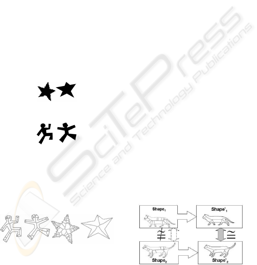
affected by small boundary variations. Here is the
question: are the two shapes so different enough if
they look similar except one has noisy boundary while
another has a smooth one (fig. 1). Another example
of two similar shapes is two human figures having dif-
ferent hands and legs positions (fig. 2).
Figure 1: Different or similar shapes?
Figure 2: Different or similar shapes?
The similarity of shapes in both cases could be
seen with a naked eye. This similarity could be
described using skeletons. However classically de-
fined continuous skeletons (Mestetski, 1998) of simi-
lar shapes could be strongly different (fig. 3). We can
see ”common” parts of skeletons of similar shapes.
But how to describe these common parts correctly?
Figure 3: Different skeletons of similar shapes.
We tried to describe strictly shapes visual simi-
larity using common skeleton parts. We considered
skeletons as a graph and used graph isomorphism to
define a similarity measure between two shapes. The
main advantage of our approach towards all known
methods is that still using skeletal graphs we don’t
forget about the boundary and define mathematically
correct shape distance.
2.3 Skeleton Isomorphism
In this section we give several basic definitions used
in our approach.
Medial axis (skeleton) of the shape Ω (Mestetski,
1998) is a set of all maximal circles inscribed in the
shape Ω.
Medial axis can be represented as a planar graph
(Choi et al., 1997), i.e.a skeletal graph. Vertices of the
skeletal graph are the centers of maximal inscribed
circles that touch the shape’s boundary ∂Ω in three or
more points. Edges of the skeletal graph touch the
shape’s boundary ∂Ω in two or more points. A skele-
ton vertex that has only one incident edge is called a
terminal vertex, more than one edge — a knot. An
edge that is incident to a terminal vertex is called a
terminal edge.
Two graphs are isomorphic G
∼
=
H if there is a
vertex mapping between them that keeps edge adja-
cency. Graph isomorphism searching is an NP-full
problem (E. M. Reingold and Deo, 1977).
Two skeletons are isomorphic if their skeletal
graphs are isomorphic and the traversal order of ter-
minal vertices is the same in both graphs.
Skeleton isomorphism can’t be used directly to
compare shapes because similar shapes have strongly
different, i.e. not isomorphic skeletons (fig. 3). Thus
we decided to find better solution.
2.4 New Approach to Compare Shapes
Using Skeletons
We propose an approach based on a simple idea
(fig. 4). For any two given shapes we find two new
shapes that are close to the given ones but have iso-
morphic skeletons.
Figure 4: Shapes with isomorphic skeletons.
Let’s denote MA(Shape) — the medial axes of the
shape (or its continuous skeleton), M — an algorithm
VISAPP 2009 - International Conference on Computer Vision Theory and Applications
238

that transforms the two given shapes into two new
shapes with isomorphic skeletons. Thus an algorithm
M should provide the following solution for any two
shapes Sh
1
and Sh
2
:
M(Sh
1
, Sh
2
) → (Sh
′
1
, Sh
′
2
) (1)
MA(Sh
′
1
)
∼
=
MA(Sh
′
2
) (2)
Moreover, new shapes Sh
′
1
and Sh
′
2
(2) should
minimally deviate from the given shapes Sh
1
and Sh
2
.
(
D
H
(Sh
1
, Sh
′
1
) → min
D
H
(Sh
2
, Sh
′
2
) → min
(3)
Where D
H
is Hausdorff distance.
This constraint (3) is very important for several
reasons. It narrows the set of solutions. We don’t need
any shapes with isomorphic skeletons. Without this
constraint any two simple shapes (not depending on
input) with isomorphic skeletons (for example, rect-
angles) could provide a solution which at least is not
correct and at most is not applicable. It defines what
we mean by ”close shapes”. It provides an opportu-
nity to estimate shape similarity as a correct distance.
Finding new shapes that satisfy both constraints
(2) and (3) among all possible plain shapes is a very
complex problem. However looking at this problem
from the skeleton side we may find an effective and
correct solution.
Let’s consider a shape representation as a set of
all maximal inscribed circles, so-called boundary-
skeletal representation (Mestetski, 1998). Using this
kind of shape representation we may directly deal
with the skeleton, change its structure and corre-
sponding radiuses. Thus we may alter the given shape
with operations affecting boundary-skeletal represen-
tation.
2.5 The Main Algorithm
We propose an algorithm M that changes the struc-
ture of two given shapes to obtain new shapes with
isomorphic skeletons (2). Two shapes are changed at
each step of the algorithm so that the distance between
the given and changed shapes is minimal (3).
The input of the main algorithm M is two
shapes Sh
1
and Sh
2
and their continuous skeletons
MA(Sh
1
) ≡ ma
1
and MA(Sh
2
) ≡ ma
2
. The output is
two new shapes Sh
′
1
and Sh
′
2
having isomorphic skele-
tons (2) and close input shapes (3).
2.5.1 Skeleton Operations
One or several operations of two types are executed at
each step of the algorithm (detailed description may
be found in (Domakhina and A.Okhlopkov, 2008)):
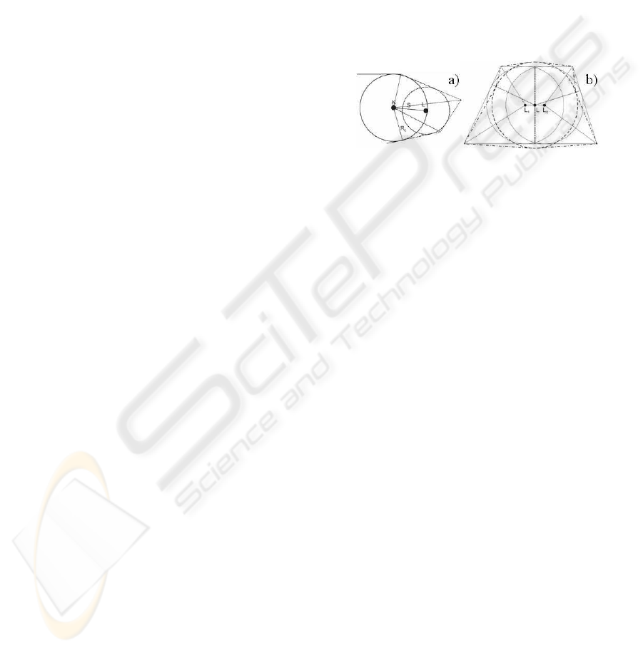
1. Terminal skeleton edges cutting (”cutting”). Cut-
ting means terminal edge’s deletion. When the
skeleton’s edge is cut all corresponding circles are
deleted as well. Cutting operation affects the in-
put figure ”angles round-up” (as shown in fig 5a).
2. Close skeleton knots merging (”merging”). This
operation merges two adjacent knots of the shape,
i.e. deletes an internal skeleton’s edge and all cor-
responding circles as well. We assign the radius
of the new knot’s circle as arithmetic mean of two
merged circles radiuses. Local shape’s changing
under merging operation is shown in figure 5b.
Figure 5: Figure’s changes during cutting and merging.
We describe an algorithm M in terms of isomor-
phic skeletons construction for two given skeletons
ma
1
and ma
2
. Remember that shape is changed dur-
ing each operation execution as described above.
2.5.2 Main Algorithm
1. Primary cutting (removing noise) of both skele-
tons ma
1
and ma
2
for a fixed valueε, i.e. obtaining
the base skeleton with a fixed accuracy ε (I.Reyer
and Mestetski, 2003). The level of noise may be
estimated depending on a shape. It may be as-
sumed to 1 if the shape is given as a raster object.
2. Equalizing the number of terminal vertices (graph
isomorphism necessary condition (E. M. Reingold
and Deo, 1977)) - secondary cutting. Let the first
skeleton (ma
1
) have more terminal vertices than
the second one (ma
2
). Skeleton’s ma
1
terminal
vertices are cut until both skeletons ma
1
and ma
2
have the same number of them.
3. Primary merging (removing small accidental
structure defects) for a fixed value ε. Internal
edges are deleted sequently while Hausdorff dis-
tance between new and input shape is less than
fixed value ε.
4. Equalizing the number of skeleton knots (graph
isomorphism necessary condition (E. M. Reingold
and Deo, 1977)) - secondary merging. This step
is executed like the second step but internal edges
are cut.
5. Sequent single operations (cutting and merging)
execution until skeleton graphs become isomor-
SHAPE COMPARISON BASED ON SKELETON ISOMORPHISM
239

phic. To satisfy algorithm’s M constraint to min-
imize shape’s deviation (3) we need to choose the
operation sequently so that deletion of the corre-
sponding edge affects the less on a shape.
2.5.3 Computational Complexity
It is easy to prove that each operation affects only lo-
cal shape changes. The computational complexity for
all algorithm’s steps is shown in table 1.
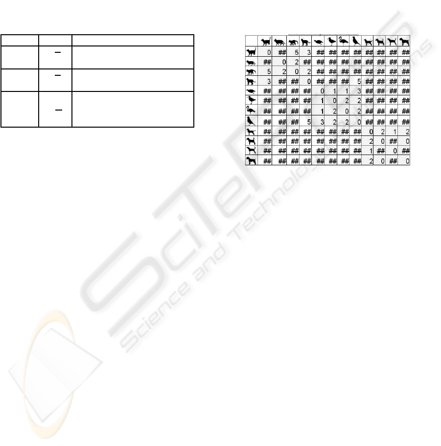
Table 1: Computational Complexity Estimation.
Step Est. The unit complexity estimated
1 and 2 O(
n
2
2
) the number of terminal vertices
3 and 4 O(
n
2
2
) the number of internal edges
the number of skeletal graph
5 O(
n
2
2
) vertices remained after
main algorithm steps 1-4
Thus maximal computational complexity could be
at most quadratic by the total number of skeleton
edges. However real complexity becomes close to lin-
ear when we use the fact that medial axis is not ab-
stract graph but a tree with the realization on a plane.
2.6 Shape Metrics
We propose two metrics based on the main algorithm.
The first one (Naive Edit-Cost) looks like edit dis-
tance (Klein et al., 2001). However we use the global
stop criterion and another algorithm. The second
(Adapted Hausdorff Metrics) is our main result. It
is a classic distance and at the same time agrees with
visual intuition. Efficiency of both metrics has been
confirmed on experiments as well.
2.6.1 ”Naive Edit-Cost” Shape Metrics
We propose the ”Naive Edit-Cost” (D
cost
) similarity
measure as a sum of all operations of the main algo-
rithm that should be executed to obtain isomorphic
skeleton. Noises of the border as well as small struc-
ture fluctuations are not taken into account. Therefore
all operations from steps 1 and 3 of the main algo-
rithm should be eliminated from the sum.
D
cost
=
∑
operations of steps 2, 4, 5 (alg. M) (4)
Figure 6 shows an example of ”Naive edit-cost” as
Shape Metrics on 12 figures of 3 classes: cats, birds
and dogs. We must mention that we added one more
stop criterion to the main algorithm. The main algo-
rithms exits when maximal of Hausdorff distances be-
tween input and changed shapes exceeds fixed value
η, i.e. max(D
H
(Sh
1
, Sh
′
1
), D
H
(Sh
2
, Sh
′
2
)) ≥ η Thus
the main algorithm may exit when isomorphism is
not found. For a pair of shapes with no found iso-
morphism we assign the distance equal to infinity ∞
which is denoted as
′
##
′
in fugure 6. It’s easy to see
that the distance between objects from one class is
less than the distance between objects from different
classes. In most cases the latter is equal to infinity
(
′
##
′
in a fig. 6).
Figure 6: An example of ”Naive edit-cost” shape metrics.
Despite the visually good results the similarity
measure defined in such a way has several essential
drawbacks:
1. Strong dependency on the algorithm’s parameters
(as we make the sum of the algorithm’s steps);
2. Discontinuity (D
cost
equals to 0,1,2,...,∞);
3. Not a distance.
Therefore we propose the better similarity mea-
sure that avoids these drawbacks. We call Adapted
Hausdorff Metrics.
2.6.2 ”Adapted Hausdorff Shape Metrics”
Hausdorff metrics (D
H
) between two shapes S
1
and
S
2
is defined as follows:
D
H
(S
1
, S
2
) = max{ρ
x∈S
1
(x, S
2
), ρ
y∈S
2
(S
1
, y)} (5)
Statement: Hausdorff Metrics (5) is a classic dis-
tance .
We define ”Adapted Hausdorff Metrics” (D
AH
)
between two shapes S
1
and S
2
as follows:
D
AH
(S
1
, S
2
) = max{D
H
(S
1
, S
2
), D
H
(S
′
1
, S
′
2
)} (6)
Where S
′
1
and S
′
2
are shapes as results of the main
algorithm M(Sh
1
, Sh
2
) → (Sh
′
1
, Sh
′
2
).
VISAPP 2009 - International Conference on Computer Vision Theory and Applications
240

Statement: Adapted Hausdorff Metrics (6) is a
classic distance.
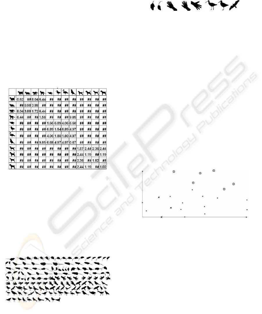
Figure 7 shows an example of ”Adapted Haus-
dorff Metrics”. We must mention that we added one
more stop criterion to the main algorithm. The main
algorithm exits when the maximal of Hausdorff dis-
tances between input and changed shapes exceeds
fixed value η, i.e. D
AH
(S
1
, S
2
) ≥ η Thus the main
algorithm may exit when isomorphism is not found.
For a pair of shapes with no found isomorphism we
assign the distance D
AH
equal to infinity ∞ which is
denoted as
′
##
′
in figure 7.
Statement: Adapted Hausdorff Metrics (6) with
additional stop criterion still remains a classic dis-
tance.
Figure 7: An example of Adapted Hausdorff Shape Metrics.
3 RECOGNITION APPLICATION
In this section we report on applying our algorithm
and proposed naive edit-cost metrics (4) and adapted
Hausdorff metrics (6) to shape recognition problems.
We took a database of total 142 binary shapes
(fig. 8). The database consists of shapes of three
classes: mice (69), hands (22) and birds (51).
Figure 8: Test data set.
We construct a feature vector for each shape by
comparing it with a set of templates. We assume that
each class has at least one template shape. These tem-
plates can be chosen accidentally or by expert.
The following 8 templates are taken: T
1
, ..., T
8
(fig. 9)
Figure 9: Test templates.
The feature vector for an object S is:
{D
cost
(S, T
1
), ..., D
cost
(S, T
8
), D
AH
(S, T
1
), ..., D
AH
(S, T
8
)}
Where D
cost
is Naive Edit-Cost (4) and D
AH
is
Adapted Hausdorff Metrics (6).
The goal was to solve a classic recognition prob-
lem: having a number of precedents (training sample)
divide testing sample objects into 3 classes.
We solve the problem using following steps:
1. Feature vector construction for each test data
shape, i.e. obtaining the feature space.
2. Accidental dividing all objects into 2 groups for
cross validation: training and testing sample.
3. Using standard methods to learn on a training
sample and estimate method’s accuracy on a test-
ing sample.
4. Repeat steps 2 and 3 to obtain impartial accuracy
estimation.
Figure 10 shows the feature space projection on a
plane with the highest dispersion.
Figure 10: Projection on a plain with the highest dispersion.
We chose several recognition methods for our ex-
periments (full methods descriptions can be found in
(Zhuravlev et al., 2005)):
Q-nearest Neighbors. The method was used as a
simple method that gives proper results when objects
are in compact groups (table 2).
Logical Regularities. The basis of Logical regular-
ities method is searching for logical regularities in
data (table 3).
Support Vector Machines. Support vector ma-
chines method is based on construction of optimal
separating hyperplane between each pair of classes.
The method is flexible and often gives the best result
comparing to other methods (table 4).
SHAPE COMPARISON BASED ON SKELETON ISOMORPHISM
241

Combined Committee Method. Committee meth-
ods use voting schemes. It’s the best solution in
case of standard methods provide errors on differ-
ent objects. We used maximum of affiliation esti-
mates for each class of the algorithms: Q-nearest
neighbors, Logical regularities and Support vector
machines. The results are perfect (table 5).
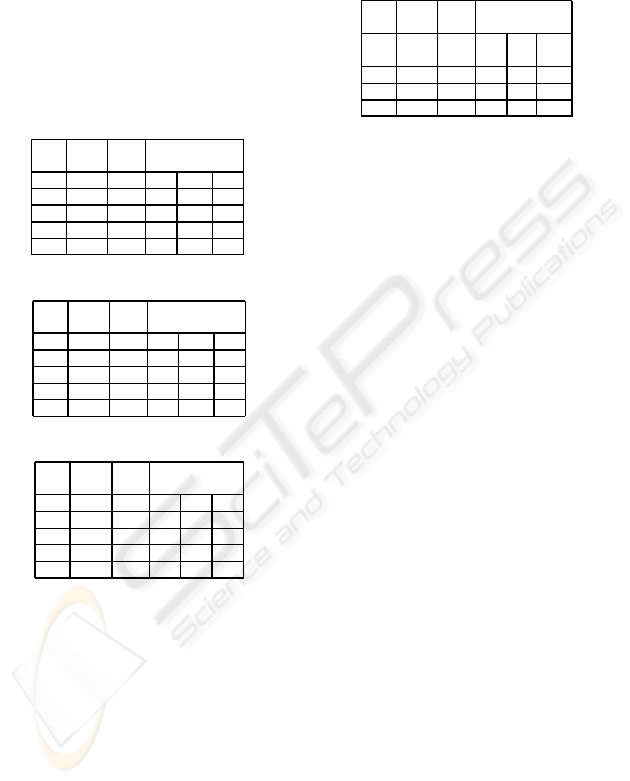
Table 2: The results of ”Q-nearest neighbors”.
Class Correct Errors Correct in classes (%)
(%) (%)
1 2 3
1 93.2 6.8 98.6 0.0 9.8
2 100.0 0.0 0.0 100.0 0.0
3 97.9 2.1 1.4 0.0 90.2
Total 95.8 4.2
Table 3: The results of ”Logical regularities”.
Class Correct Errors Correct in classes (%)
(%) (%)
1 2 3
1 95.8 4.2 98.6 0.0 5.9
2 91.7 8.3 0.0 100.0 3.9
3 97.8 2.2 1.4 0.0 88.2
Total 95.1 4.2
Table 4: The results of ”Support vector machines”.
Class Correct Errors Correct in classes (%)
(%) (%)
1 2 3
1 94.4 5.6 98.6 9.1 3.9
2 100.0 0.0 0.0 90.9 0.0
3 98.0 2.0 1.4 0.0 96.1
Total 96.5 3.5
As a result the only incorrectly classified object
is a mouse that has been referred to a ”birds” class.
Thus we proved that our approach has been imple-
mented successfully. Reported experiments showed
very good results in recognition application.
Our future work includes enlarging the test data
base and finding a real application for our approach.
4 CONCLUSIONS
A new approach to shape comparison problem is pre-
sented in the paper. An approach is based on skeleton
isomorphism, in particular, on finding close shapes
with isomorphic skeletons. We proposed the shape
comparison algorithm and two skeleton metrics based
Table 5: The results of combined committee method.
Class Correct Errors Correct in classes (%)
(%) (%)
1 2 3
1 100.0 0.0 98.6 0.0 0.0
2 100.0 0.0 0.0 100 0.0
3 98.1 1.9 1.4 0.0 100.0
Total 99.3 0.7
on shapes with isomorphic continuous skeletons con-
struction. The proposed shape comparison algorithm
differs from existing ones by correctly defined dis-
tance corresponding with visual intuition. The exper-
iments showed very good results in recognition appli-
cations. Thus we confirmed that our theoretical result
does not contradict practical experiments.
ACKNOWLEDGEMENTS
Work is supported by the RFBR project
08− 01 − 00670. We thank our supervisor pro-
fessor L. Mestetski for his help.
REFERENCES
Choi, H. I., Choi, S. W., and Moon, H. P. (1997). Mathe-
matical theory of medial axis transform. Pacific.J. of
Math, 181(1):57–88.
Domakhina, L. and A.Okhlopkov (2008). Isomorphic skele-
tons of raster images. In 18th International Confer-
ence Graphicon-2008.
E. M. Reingold, J. N. and Deo, N. (1977). Combinatorial
Algorithms, Theory and Practice. P.
I.Reyer and Mestetski, L. (2003). Continuous skeletal rep-
resentation with fixed accuracy. In 13th Int. Confer-
ence Graphicon-2003.
Klein, P. N., Sebastian, T. B., and Kimia, B. B. (2001).
Shape matching using edit-distance: An implementa-
tion. In The twelfth annual ACM-SIAM symposium on
Discrete algorithms, pages 781 – 790.
Liu, T. and Geiger., D. (1999). Approximate tree matching
and shape similarity. In ICCV.
Mestetski, L. (1998). Continuous skeleton of raster images.
In 8th Int. Conference Graphicon-1998.
Sebastian, T. B. and Kimia., B. B. (2001). Curves vs skele-
tons in object recognition. In Division of Engineering,
Brown University. Providence, RI 02912, USA.
Tanase, M. (2005). Shape Decomposition and Retrieval.
PhD thesis, Utrecht University.
Zhuravlev, J., V.Ryazanov, and O.Senko (2005). Recog-
nition. Mathematical Methods. Practical Solutions.
Phasis Edition, Moscow.
VISAPP 2009 - International Conference on Computer Vision Theory and Applications
242