ON THE SOLUTIONS OF NP-COMPLETE PROBLEMS

BY MEANS OF JNEP RUN ON COMPUTERS

Emilio del Rosal García

1,2

, José Miguel Rojas Siles

, Rafael Núñez Hervás

Carlos Castañeda Marroquín

and Alfonso Ortega de la Puente

Escuela Politécnica Superior de la Universidad San Pablo CEU, Madrid, Spain

Departamento de Ingenieria Informática, Universidad Autónoma de Madrid, Madrid, Spain

Keywords: NEP, Natural computing, Multi agent systems, Simulation.

Abstract: We have used jNEP (a JAVA simulator of a natural computing device named Networks of Evolutionary

Processors) to solve some cases of well-known NP-complete problems. We have followed the most relevant

papers in the literature. In this paper, we describe the difficulties found in this process and some conclusions

about the design, the simulation and some useful tools for NEPs.

1 INTRODUCTION

1.1 Bio Inspired Computational

Devices

The so-called natural computing devices (such as

multiagent systems, P systems, cellular automata, L

systems and NEPs) are formal complex systems that

are able to compute and could, therefore, be used as

computers. All of them share two main

characteristics: their inspiration in the way in which

Nature efficiently solves complex tasks and an

intrinsic parallelism that makes it possible to

develop algorithms which improve the temporal

performance of classic von Neumann architectures.

This paper is specifically devoted to NEPs. As they

could be considered as an alternative to the von

Neumann architecture, a great research effort is

currently being made to study the necessary tools to

program them. We tackle this goal in two forms:

studying the techniques to design NEPs which solve

given problems, and developing and using a real

hardware/software platform to run these NEPs.

1.2 NP-Complete Problems

In this section we informally introduce this topic. A

formal description could be found in any manual

(Garey and Johnson, 1979) on complexity and is out

of the scope of this paper.

NP may be informally defined as the set of

decision problems that can be solved in polynomial

time on a no deterministic Turing machine.

An NP problem is also complete if and only if

every other problem in NP can be easily (in

polynomial time) transformed into it.

Polynomial performance on a non-deterministic

Turing machine frequently corresponds to at least

exponential performance on a deterministic Turing

machine. Classical von Neumann computers can be

considered the closest implementation of

deterministic Turing machines.

Even more informally, the reader can consider a

non-deterministic Turing machine as a set of as

many Turing machines as needed, searching in

parallel for a solution of the problem. Such a device

will stop as soon as the first solution is found. Each

Turing machine is expected to check its solution in

polynomial time. In the previous statement, “as

many Turing machines as needed” usually means

“an exponential number of machines”.

The reader can easily understand that if the same

work has to be done by a single Turing machine, it

has to check each of the possible solutions (an

exponential amount of them) in a polynomial time,

which results in a final exponential performance.

1.3 NEPs

NEP (Castellanos, 2001), (Castellanos, 2003) stands

for Network of Evolutionary Processors. NEPs are

605

del Rosal Garc

ıa E., Miguel Rojas Siles J., N

nez Herv

as R., Casta

neda Marroqu

ın C. and Ortega de la Puente A. (2009).

ON THE SOLUTIONS OF NP-COMPLETE PROBLEMS BY MEANS OF JNEP RUN ON COMPUTERS.

In Proceedings of the International Conference on Agents and Artiﬁcial Intelligence, pages 605-612

 SciTePress

an abstract model of distributed/parallel symbolic

processing inspired by biological cells. They

distribute a set of simple string processors in the

nodes of a fixed graph. Processors contain strings of

symbols, change them in a predefined way and filter

them to communicate some of these words to the

other processors of the graph.

Despite the simplicity of each processor, the

entire net can efficiently carry out very complex

tasks. Many different works demonstrate the

computational completeness of NEPs (Csuhaj-Varju,

2005), (Manea, 2007) and their ability to solve NP

problems with linear or polynomial resources

(Manea, 2006), (Castellanos, 2001). The emergence

of such a computational power from very simple

units acting in parallel is one of the main interests of

NEPs.

A NEP is built from the following elements:

a) a set of symbols which constitutes the

alphabet of the words which are

manipulated by the processors,

b) a set of processors,

c) an underlying graph where each vertex

represents a processor and the edges

determine which processors are connected

so they can exchange words,

d) an initial configuration defining which

words are in each processor at the

beginning of the computation and

e) one or more stopping rules to halt the NEP.

An evolutionary processor has three main

components:

a) a set of evolutionary rules to modify its

words,

b) some input filters that specify which words

can be received from other processors and

c) some output filters that delimit which

words can leave the processor to be sent to

others.

The variants of NEPs mainly differ in their

evolutionary rules and filters. They perform very

simple operations, like altering the words by

replacing all the occurrences of a symbol by another,

or filtering those words whose alphabet is included

in a given set of words.

NEP's computation alternates evolutionary and

communication steps: an evolutionary step is always

followed by a communication step and vice versa.

Computation follows the scheme below: when

the computation starts, every processor has a set of

initial words.

At first, an evolutionary step is performed: the

rules in each processor modify the words in the same

processor. Next, a communication step forces some

words to leave their processors and also forces the

processors to receive words from the net.

The communication step depends on the

constraints imposed by the connections and the

output and input filters.

The model assumes that an arbitrary number of

copies of each word exists in the processors,

therefore all the rules applicable to a word are

actually applied, resulting in a new word for each

rule.

The NEP stops when one of the stopping

conditions is met, for example, when the set of

words in a specific processor (the ouput node of the

net) is not empty. A detailed formal description of

NEPs can be found in (Castellanos, 2003), (Csuhaj-

Varju, 2005) or (Manea, 2007).

1.4 Clusters of Computers running

Java

Java is currently one of the most popular object

oriented programming languages. Java may be

slower than other programming languages for

computation-intensive problems. Nevertheless it is

possible to run Java programs on a cluster of

computers by means of a special Distributed Java

Virtual Machine (DJVM), which supports parallel

execution of Java threads. In this way, a

multithreaded Java application runs on a cluster just

as if it were running on a single machine, but with

the same performance as a big multi-processor

machine.

DJVMs are not included in the Sun's standard

Java distributions. There are several different kinds

of DJVM, for example: Java-Enabled Single-

System-Image Computing Architecture 2

(JESSICA2), the cluster virtual machine for Java

developed by IBM (IBM cJVM), Proactive PDC

(Proactive), DO! (Launay 97), JavaParty

(JavaParty), Jcluster (Jcluster), MPJ Express (MPJ),

and Terracota (Terracota, 2008).

The simulator used in this paper has been

developed with both, standard JVM and JavaParty.

2 JNEP

In a previous work (Rosal, 2008) we have explained

the reasons to develop a NEP simulator to be run in

a cluster of computers.

ICAART 2009 - International Conference on Agents and Artificial Intelligence

606

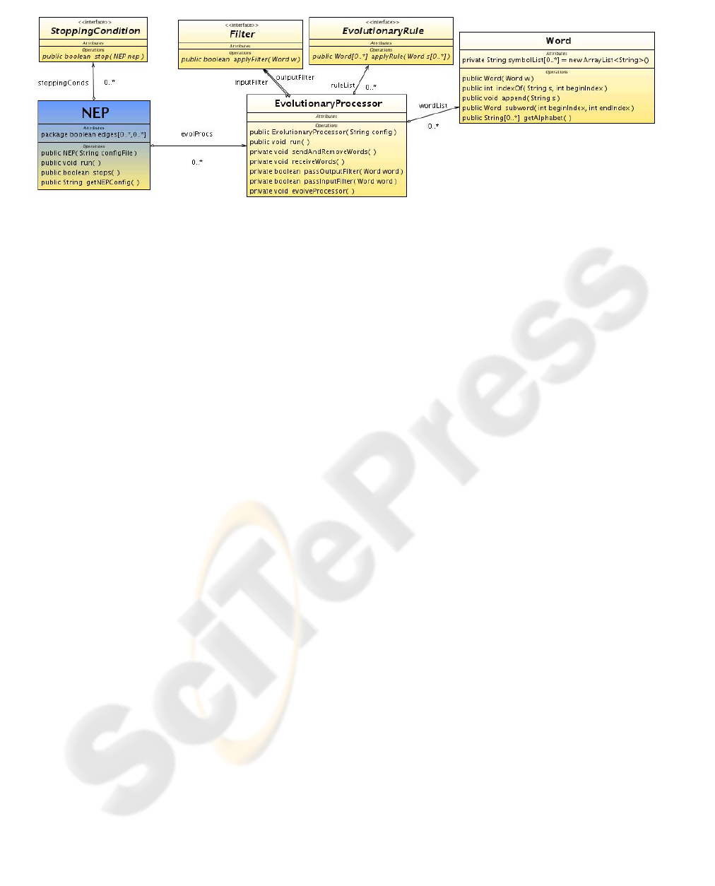
Figure 1: Simplified class diagram for jNEP.

jNEP offers an implementation of NEPs as

general, flexible and rigorous as possible. This is not

an obvious goal, because we have observed that

different authors understand the model definition in

slightly different ways. These subtle differences

imply, nevertheless, hard to overcome problems in

the development of a computer application that

implements all of them.

As shown in figure 1, the design of the NEP

class mimics the NEP model definition. In jNEP, a

NEP is composed of evolutionary processors and an

underlying graph (attribute edges) to define the net

topology and the allowed inter processor

interactions. The NEP class coordinates the main

dynamic of the computation and rules the processors

(instances of the EvolutionaryProcessor class),

forcing them to perform alternate evolutionary and

communication steps. It also stops the computation

when needed.

The core of the model includes these two classes,

together with the Word class, which handles the

manipulation of words and their symbols.

jNEP is kept as general and rigorous as possible

by means of the following mechanisms: Java

interfaces and the development of different versions

to widely exploit the parallelism available in the

hardware platform. Further details can be found in

(Rosal, 2008) and at (http://jnep.e-delrosal.net).

jNEP currently has two lists of choices

(concurrency approach and platform) to select the

parallel/distributed platform on which it runs (jNEP

versions for any possible combination of them are

available in http://jnep.e-delrosal.net).

Concurrency is implemented with two different

Java approaches: Threads and Processes.

The supported platforms are standard JVM and

clusters of computers (by means of JavaParty).

jNEP reads the definition of the NEP that is

being simulated from a configuration file that

follows XML conventions. Roughly speaking the

configuration file contains special tags for any

relevant component in the NEP (alphabet, stopping

conditions, the complete graph, each edge, each

evolutionary processor with its rules, filters and

initial contents).

Although some fragments of these files will be

shown in these pages, all the configuration files

mentioned in this paper can be found at

(http://jnep.e-delrosal.net). Despite the complexity

of these XML files, the interested reader can see that

these tags and their attributes have self-explaining

names and values.

3 SOLVING NP-COMPLETE

PROBLEMS WITH JNEP

In our previous work (Rosal, 2008) we showed, as

an example, how to solve the propositional logic

SAT problem for three variables by means of a NEP

with a kind of special rules (splicing) taken from

(Manea, 2007).

In this work we show how jNEP has been used to

solve some instances of other two well-known NP-

complete problems: the Hamiltonian path problem

and the 3-coloring problem.

3.1 Hamiltonian Path Problem

This well-known NP-complete problem searches an

undirected graph for a Hamiltonian path, that is, one

that visits each vertex exactly once.

In his work (Adleman, 1994) Adleman proposed

a way to solve this problem with polynomial

resources by means of DNA manipulations in the

laboratory. Figure 2 shows the graph used by

Adleman. The solution is in this case obvious (path

ON THE SOLUTIONS OF NP-COMPLETE PROBLEMS BY MEANS OF JNEP RUN ON COMPUTERS

607

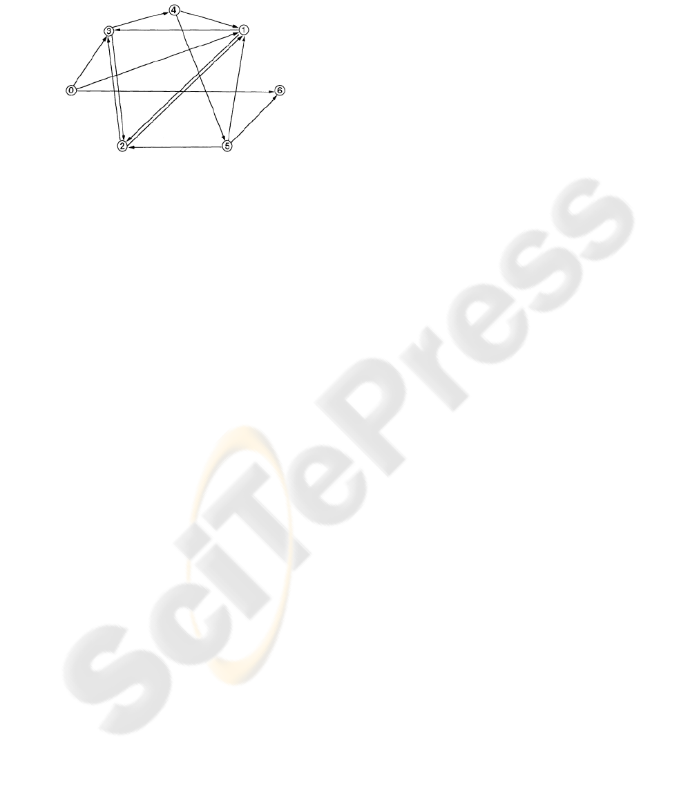
0-1-2-3-4-5-6) Despite its simplicity, Adleman

described a general algorithm applicable to almost

ny graph with the same performance.

Figure 2: Graph studied by Adleman.

an’s algorithm can be summarized as

hose paths that begin and end in the

paths that contain exactly the

ose paths that contain some node

remaining paths are solutions for the

pro

definition of the stopping

the initial content of

the string received from the

ble

ng filters by

x regular expression or a greater

l). Some of their sections are explained

bel

example defines the

tent of node 0 in the

are defined as follows

of the alphabet

and no string is forb e

_3_4_5_6"

ingContext="" />

/FILTERS>

n empty node

to this string

ext steps only nodes 1,

e respectively i_0_1, i_0_3 and

Adlem

foll ws:

1. Generating randomly all the possible paths.

2. Selecting t

pro er nodes.

3. Selecting only the

tota number of nodes.

4. Removing th

more than once.

5. The

blem.

The present work follows a similar approach.

• The NEP graph is very similar to the one

studied above: an extra node is added to

ease the

condition.

• The set {i,0,1,2,3,4,5,6} is used as the

alphabet. Symbol i is

the initial vertex (v

)

• Each node (except the final one) adds its

number to

network.

• Input and output filters are defined to allow

the communication of all the possi

words without any special constraint.

• The input filter of the final node excludes

any string which is not a solution. It is easy

to imaging a regular expression for the set

of solutions (those words with the proper

length, the proper initial and final node and

where each node appears only once). The

NEP basic model allows defini

means of regular expressions.

• It is also easy to devise a set of additional

nodes that performs the previous filter

following Adleman’s checks (proper

beginning and end, proper length, and

number of occurrences of each node). For

the shake of simplicity we have used

explicitly the solution word

(i_0_1_2_3_4_5_6) instead of a more

comple

NEP.

The reader will find at http://jnep.e-delrosal.net

the complete XML file for this problem

(Adleman.xm

ow:

• The XML file for this

alphabet with this tag

• the initial con

following way

• The rules for adding the number of the

node to its string

(here for node 2)

<RULE ruleType = "insertion"

actionType = "RIGHT"

ymbol = "2" newSymbol="" />

• There are several ways of defining filters

for the desired behavior (to allow the

communication of all the possible words

without any special constraint). We have

used only the permitted input and output

filters. A string can enter a node if it

contains any of the symbols

idd n.

<INPUT type="2"

permittingContext="i_0_1_2

forbiddingContext="" />

<OUTPUT type="2"

permit ingContext="i_0_1_2t

forbidd

The behavior of the NEP is sketched as follows:

1. In the initial step the only no

is 0 and contains the string i

2. After the first step, 0 is added

and thus, node 0 contains i_0

3. This string is moved to the nodes connected

with node 0. In the n

and 6 contain i_0.

4. These nodes add their number to the

received string. In the next step their

contents ar

i_0_6

ICAART 2009 - International Conference on Agents and Artificial Intelligence

608

5. This process is repeated as many times as

needed to produce a string that meets the

conditions of the solution. In this final step

NEP model poses

som

a set of strings. This mechanism contains

obv

eneral agreement

of the researchers to ease and simplify the

have

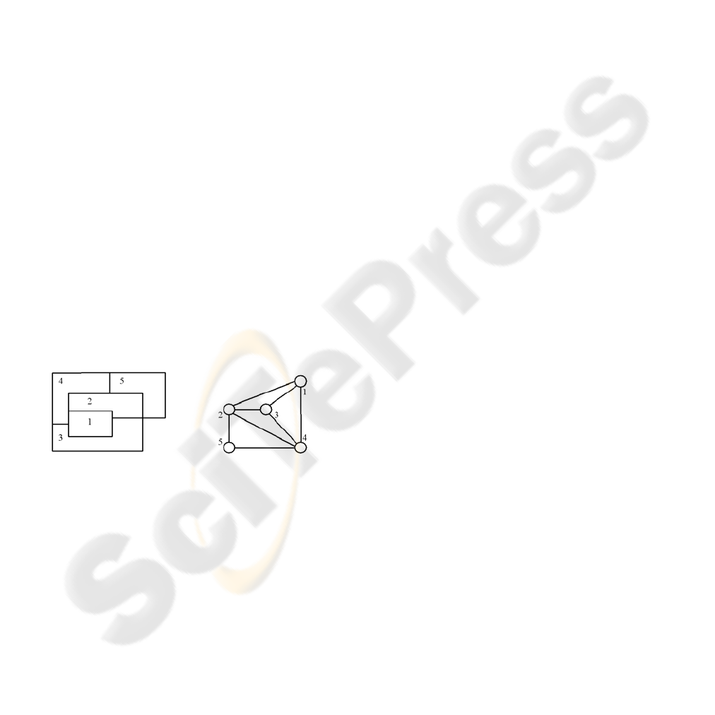
ws one of the examples studied

in this paper. It is ease to prove that there is no

solution to this map.

the solution string (i_0_1_2_3_4_5_6 is

sent to node 7 and the NEP stops.

The definition of filters in

e difficulties to the design of NEPs and, thus, to

the development of a simulator.

These filters are defined (Castellanos, 2001) and

(Castellanos, 2003) by means of two couples of

filters (forbidden and allowed) to each operation

(input and output). There exist, in addition, different

ways of combining and apply the filters to translate

them into

ious redundancies that make it difficult to design

NEPs.

It could be advisable a more g

development of NEPs simulators.

3.2 Coloring Problems

This problem introduces a map whose regions

be colored with only three colors, and with a

different one for each pair of adjacent regions.

We have used the NEP defined in (Castellanos,

2003). The map is translated into an undirected

graph whose nodes stand for the regions and whose

edges represent the adjacency relationship between

regions. Figure 3 sho

Figure 3: Example of a map and its adjacency graph. In

this case, there is no solution for the 3-colorability

pro

aph. These nodes perform the tasks

utlined below. Next paragraphs describe them with

the map are grouped in three couples (one

cate with the set of

performs this task in the

associated with the pair of

first

ode of the

e are red-blue

and red-green.

he complete NEP could be

. In this way, the process

e to see that these strings are

w to

escribe the above behavior with more detail:

abet of the NEP is defined as

follows:

r4_g4_b5_r5_g5_B1_R1_G1_B2_R2_G2_B3_R3_

blem.

The NEP has a complete graph with two special

nodes (for the initial and final steps) and a set of

seven nodes associated to each edge of the

adjacency gr

more detail:

• The initial (final) node is responsible of

starting (stopping) the computation.

• The seven nodes associated with an edge of

for each color). There is, in addition, a

special node to communi

nodes of the next edge.

• Each couple is responsible of the main

operation in the NEP: to check that a

coloring constraint is not violated for the

current edge. It

following way:

o Let us suppose that the color red is

the one

nodes.

o The first node in the NEP

associates the color red to the

node of the edge in the map.

o The second node in the NEP

simultaneously keeps all the

allowed coloring (two, in this

case) for the second n

edge: (blue and green)

o It is clear that the only acceptable

colorings for this edg

The behavior of t

sketched as follows:

1. The initial node generates all the possible

assignment of colors to all the regions in

the map and adds a symbol to identify the

first edge to be checked. These strings are

communicated to all the nodes of the graph.

2. The set of nodes associated to each edge

accepts only the strings marked with the

symbol of the edge. These nodes remove all

the strings that violate the coloring

constraint for the regions of the edge. One

special node in the set replaces the edge

mark with that which corresponds to the

next edge

ntinues.

3. The final node of the NEP collects the

strings that satisfy the constraints of all the

edges. It is eas

the solutions.

Some fragments of the XML file for this

example (3Coloring.xml) are shown belo

• The alph

<ALPHABET

symbols="b1_r1_g1_b2_r2_g2_b3_r3_g3_b4_

ON THE SOLUTIONS OF NP-COMPLETE PROBLEMS BY MEANS OF JNEP RUN ON COMPUTERS

609

G3_B4_R4_G4_B5_R5_G5_a1_a2_a3_a4_a5_X1_

X2_X3_X4_X5_X6_X8_X9"/>

• This alphabet contains the following

subsets of symbols:

o {a1,…,a5} represents the initial

situation of the regions

(uncolored).

o {b1, r1, g1,…, b5, r5, g5}

represents the assignment of the

colors to the regions.

o {B1, R1, G1,… B5, R5, G5} is a

copy of the previous set to be used

while checking the constraint

associated with a couple of

adjacent regions.

• The string contained in the initial node at

the beginning represents the complete map

uncolored and the number of the first edge

to be tackled (X1)

• The rules of the initial node assign all the

possible colors to all the regions. The

following rules refer to the second region:

<RULE ruleType = "substitution"

actionType = "ANY"

symbol="a2" newSymbol="b2"/>

<RULE ruleType="substitution"

actionType="ANY"

symbol="a2" newSymbol="r2"/>

<RULE ruleType="substitution"

actionType="ANY"

symbol="a2" newSymbol="g2"/>

• The node in the NEP that assigns a color

(red, in this case) to the first region (1 in the

example) of an edge in the map uses the

following rule:

<RULE ruleType="substitution"

actionType="ANY" symbol="r1"

newSymbol="R1"/>

• The other node ensures that the adjacent

region (2 in this case) has a different color

by means of these rules:

<RULE ruleType="substitution"

actionType="ANY"

symbol="b2"

newSymbol="B2"/>

<RULE ruleType="substitution"

actionType="ANY" symbol="g2"

newSymbol="G2"/>

• The node used for starting the process in

the next edge removes any special

(capitalized) color symbol and sets the edge

marking to the next one. The following

rules correspond to the first edge

<RULE ruleType="substitution"

actionType="ANY" symbol="R1"

newSymbol="r1"/>

<RULE ruleType="substitution"

actionType="ANY" symbol="B1"

newSymbol="b1"/>

<RULE ruleType="substitution"

actionType="ANY" symbol="G1"

newSymbol="g1"/>

<RULE ruleType="substitution"

actionType="ANY" symbol="R2"

newSymbol="r2"/>

<RULE ruleType="substitution"

actionType="ANY" symbol="B2"

newSymbol="b2"/>

<RULE ruleType="substitution"

actionType="ANY" symbol="G2"

newSymbol="g2"/>

<RULE ruleType="substitution"

actionType="ANY" symbol="X1"

newSymbol="X2"/>

• We have found difficulties when applying

the input and output filters as they are in

(Castellanos 2003). We have previously

explained our opinion on the advisability of

a greater standardization to minimize this

situations.

• Notice that the nodes associated with the

last edge (in this case with the number 8)

mark its strings with the following number

that does not correspond with any edge in

the graph (9 in our example). This is

important for the design of the final node.

• A special node of the NEP checks the

stopping condition (Non Empty Node

Stopping Condition). This final node only

accepts strings with the corresponding mark

(one that does not correspond to any edge

in the adjacency graph).

Figure 4 shows other map that could be colored

with 3 colors. Splitting region 3 and 4 in figure 3

generates this map. Figure 4 also summarizes the

sequence of steps for one of the possible solutions. It

is worth noticing that all the solutions are

ICAART 2009 - International Conference on Agents and Artificial Intelligence

610

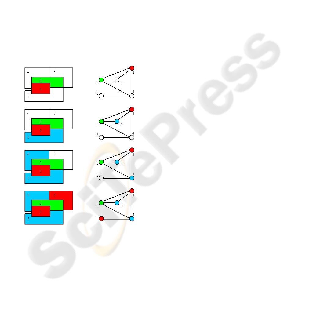
simultaneously kept in the configurations of the

NEP.

The behavior of the NEP for this map could be

summarized as follows:

• The initial content of the initial node is

a1_a2_a3_a4_a5_X1.

• This node produces all the possible

coloring combinations. In the second step

of the computation, for example, it contains

the following strings:

b1_a2_a3_a4_a5_X1 r1_a2_a3_a4_a5_X1

g1_a2_a3_a4_a5_X1 a1_b2_a3_a4_a5_X1

a1_r2_a3_a4_a5_X1 a1_g2_a3_a4_a5_X1

a1_a2_b3_a4_a5_X1 a1_a2_r3_a4_a5_X1

a1_a2_g3_a4_a5_X1 a1_a2_a3_b4_a5_X1

a1_a2_a3_r4_a5_X1 a1_a2_a3_g4_a5_X1

a1_a2_a3_a4_b5_X1 a1_a2_a3_a4_r5_X1

a1_a2_a3_a4_g5_X1

Figure 4: Sequence of steps in the solution of a 3-coloring

problem by jNEP.

• The NEP still needs a few more steps to get

all the combinations.

• After that, the coloring constraints are

applied simultaneously to all the possible

solutions and those assignments that violate

some constraint are removed. We describe

below a sequence of strings generated by

the NEP that corresponds to the solution

graphically shown in figure 4:

o r1_g2_b3_b4_r5_X1 is generated

in the initial steps.

o After checking the 1st edge

(regions 1 and 2) the NEP contains

these two strings

R1_g2_b3_b4_r5_X1 and R1_G2_b3_b4_r5_X1

o After checking the 2nd edge

(regions 1 and 3)

R1_g2_B3_b4_r5_X2

o And after checking the edges 3, 4,

5, 6 and 8 (remember that edge 7

was removed to make the map

colorable) associated respectively

with the pairs of regions 1-4, 2-3,

2-4, 2-5 and 4-5, the following

strings are in the NEP:

R1_g2_b3_B4_r5_X3 r1_G2_B3_b4_r5_X4

r1_G2_b3_B4_r5_X5 r1_G2_b3_b4_R5_X6

r1_g2_b3_B4_R5_X8

o Finally, the complete solution is

found

r1_g2_b3_B4_R5_X9 and r1_g2_b3_b4_r5_X9

• This NEP processes all the solutions at the

same time. It removes all the coloring

combinations that violate any constraint.

The final node contains in the last step all

the solutions found.

(Castellanos, 2003) describes one of the kinds of

NEPs (simple NEPs) that is simulated by jNEPs. As

we have briefly mentioned before, we have observed

that the authors have used slightly different filters

for the 3-coloring problem. We could not use these

filters and we had to change some of them (most of

the output filters) in order to get a proper behavior of

the NEP. The complete XML file is available at

http://jnep.e-delrosal.net.

4 CONCLUSIONS AND

FURTHER RESEARCH LINES

We have tackled the solution of several NP-

complete problems found in the literature by means

of jNEP. We have observed that there exist different

ways of implementing the same formal model,

mainly with respect to input and output filters. These

open aspects have to be defined when the model is

implemented to solve given problems. We conclude

that simulation needs both: a formal definition and

ON THE SOLUTIONS OF NP-COMPLETE PROBLEMS BY MEANS OF JNEP RUN ON COMPUTERS

611

also some standardization in the way in which

different authors particularize these open aspects in

the implementation of their own NEPs. These

differences make it very difficult to fully understand

the behavior of the proposed NEPs as well as their

simulation. Although we have not found any

significant mistake in the simulation of the formal

model, we had to modify and improve jNEP in

several subtle details in order to ease the handling of

the NEPs described in the literature.

We have also identified some common

techniques to these different NP problems. They

suggest us some tools that could be added to jNEP to

increase the comfort of the NEPs designer. In the

future we plan to develop a more abstract input

format. For example, most of the NEPs defined to

solve NP problems uses complete graphs. The

current XML configuration file explicitly defines

each edge, which implies a big amount of tedious

and mechanical work. It will be very useful some

automatic mechanism to do this task.

It could be also very useful adding some

diagnose tool to check the correctness of the NEPs.

It is worth noticing that jNEP is just a block that

will be used to build more complex applications.

One of them is a full graphic simulation

environment for NEPs that ease their design to solve

given problems. Our research group is also

interested in some evolutionary techniques to

automatic design NEPs. jNEP will be used as a part

of the fitness function that this kind of algorithms

needs.

ACKNOWLEDGEMENTS

This work was supported in part by the Spanish

Ministry of Education and Science (MEC) under

Project TSI2005-08225-C07-06. We want to thank

to Manuel Alfonseca his help in the preparation of

this paper.

REFERENCES

Adleman, 1994. Molecular Computation of Solutions To

Combinatorial Problem. In Science, 266: 1021-1024,

(Nov. 11) 1994.

Castellanos, J., Martin-Vide, C., Mitrana, V., and

Sempere, J.M., 2001. Solving NP-Complete Problems

With Networks of Evolutionary Processors In

Connectionist Models of Neurons, Learning Processes

and Artificial Intelligence: 6th International Work-

Conference on Artificial and Natural Neural

Networks, IWANN 2001 Granada, Spain, June 13-15,

Proceedings, Part I, 2001.

Castellanos, J., Martin-Vide, C., Mitrana, V., and

Sempere, J.M., 2003. Networks of evolutionary

processors. In Acta Informatica, 39(6-7):517-529,

2003.

IBM cJVM,

http://www.haifa.il.ibm.com/projects/systems/cjvm/in

dex.html

Csuhaj-Varju, E., Martin-Vide, C., and Mitrana, V., 2005.

Hybrid networks of evolutionary processors are

computationally complete. In Acta Informatica, 41(4-

5):257-272, 2005

Garey, M.R., Johnson, D.S., 1979. Computers and

intractability: a guide to the theory of NP-

completeness. New York: W.H. Freeman. ISBN 0-

7167-1045-5.

JavaParty http://wwwipd.ira.uka.de/JavaParty/

Jcluster http://vip.6to23.com/jcluster/

JESSICA2 http://i.cs.hku.hk/~wzzhu/jessica2/index.php

Launay, P., Pazat J.L., 1997. A Framework for Parallel

Programming in Java. INRIA Rapport de Recherche

Publication Internet - 1154 decembre 1997 - 13 pages

Manea, F., Martin-Vide, C., and Mitrana, V., 2007.

Accepting networks of splicing processors:

Complexity results. In Theoretical Computer Science,

371(1-2):72-82, February 2007.

Manea, F., Martin-Vide, C., and Mitrana, V., 2006. All

np-problems can be solved in polynomial time by

accepting networks of splicing processors of constant

size In DNA Computing, pages 47-57, 2006.

MPJ http://mpj-express.org/

ProActive http://www-sop.inria.fr/sloop/javall/

del Rosal, E. del, Nuñez, R., Castañeda, C., Ortega, A.,

2008. Simulating NEPs in a cluster with jNEP. In

International Conference on Computers,

Communications and Control, ICCCC 2008, to be

held in European Union, Romania, Oradea, Băile

Felix (Spa), May 15-17, 2008. Proceedings.

Terracotta, Inc, 2008. The Definitive Guide to Terracotta:

Cluster the JVM for Spring, Hibernate and POJO

Scalability (The Definitive Guide), Apress Publishing.

Expert's Voice in Open Source Series June 2008.

ISBN:9781590599860.

ICAART 2009 - International Conference on Agents and Artificial Intelligence

612