Automated Segmentation and Clinical Information on

Dementia Diagnosis

A. Conci

, A. Plastino

, A. S. Souza

, C. S. Kubrusly

, D. M. Saade

and F. L. Seixa

UFF, Computer Institute, Passo da Patria 156, 24210 240 Niteroi, RJ, Brazil

Radiology Department, LABS-Rede D´Or, 22032 011 Rio de Janeiro, RJ, Brazil

PUC/RJ, Eletrical Engineering Department, R. Marques de S. Vicente 225

22453-900, Rio de Janeiro, RJ, Brazil

UFF, Telecommunications Engineering Department, Passo da Patria 156

24210 240 Niteroi, RJ, Brazil

Abstract. This work intends to predict the clinical dementia rating (CDR)

based on human brain volumetric segmentation measures from magnetic reso-

nance (MR) images. These brain measures were extracted using an automated

image segmentation method based on morphometry study and considering

brain anatomical atlas. The prediction was achieved by Bayesian classifier. The

classifier training was performed on 371 individuals from Open Access Series

of Imaging Studies (OASIS) dataset. MR images and clinical information (in-

cluding the Clinical Dementia Rating score) of each case are available on

OASIS dataset. Experimentation results were assessed using true-positive rate.

The final purpose of this work is to design a computer-aided diagnostic system

that could be able to detect precociously neurodegenerative disorders, allowing

early therapeutic interventions.

1 Introduction

Neurodegenerative disorders, such as multiple sclerosis, Alzheimer, Huntington and

Parkinson diseases, are characterized by neuronal cell loss or dysfunction [1]. It is

estimated that these disorders affect 11 million individuals, aged 60 years or older [1].

Alzheimer’s disease (AD) represents the most common cause of dementia [2]. AD

diagnostic criteria are based on the National Institute of Neurology Communicative

Disorders and Stroke-Alzheimer’s Disease and Related Disorders Association

(NINCDS-ADRDA) criteria [3]. The Clinical Dementia Rating (CDR) scale is a

global dementia staging instrument developed by the Memory and Aging Project [4].

CDR presents 5 scores: 0 (no dementia), 0.5 (questionable), 1 (mild), 2 (moderate)

and 3 (severe). Agreement of CDR score with NINCDS-ADRDA’s criteria achieves

86% for sensitivity and 100% for specificity [5]. A previous validation of this scale in

Brazil was carried out achieving 91% sensitivity and 100% specificity [6]. Structures

located in the medial temporal lobe, such as hippocampus and the parahippocampal

Conci A., Plastino A., Souza A., Kubrusly C., Saade D. and Seixas F. (2009).

Automated Segmentation and Clinical Information on Dementia Diagnosis.

In Proceedings of the 1st International Workshop on Medical Image Analysis and Description for Diagnosis Systems, pages 33-42

DOI: 10.5220/0001811200330042

 SciTePress

gyrus are the first to manifest atrophy in AD [7]. Numerous studies and applications

of brain volumetric measurements to early detect neurodegenerative disorders and to

follow-up the patient disease progress have been presented [8]. It has been suggested

that the atrophy of medial temporal lobe structures can predict AD risk [8]. These

structures can be evaluated by magnetic resonance (MR) or, less accurately, com-

puted tomography (CT) imaging. Our work proposes the use of automated segmenta-

tion methods and classifiers models to analyze brain structure volumes on MR images

and predict patient’s CDR scores. The automated segmentation algorithm is based on

the Voxel-Based Morphometry (VBM) method [9]. The classifier model adopted was

the naïve Bayesian approach [10], assuming that brain structure volume values are

independent. 371 MR T1-weighted images from distinct patients, aged 18 to 96

years-old, were used in our practical experiments. This work extends the ideas pre-

sented in [11]. In next section the used segmentation procedure is presented. Section

3 considers the experiments and section 4 presents its conclusions.

2 Segmenting Brain Structures

Manual volumetric techniques are expensive and time-consuming. Some segmenta-

tion of medial temporal structures has being reported as taking about 75 minutes per

exam and patient [12]. Moreover it results great variability of final medial temporal

lobe volume [12-14]. Aiming to reduce the excessive time consumed and to standard-

ize its volumetric acquisition method, decreasing inter and intra-personal volumes

variability, automated image analyzing have been proposed [15]. This technique al-

lows brain tissue segmentation and volume assessment without direct human inter-

vention. Voxel-Based Morphometry (VBM) computes a customized template and the

prior probability map from a population. The map was computed by segmenting the

normalized images into grey matter (GM), white matter (WM) and cerebrum-spinal

fluid (CSF), thus averaging the segmented image and finally obtaining the customized

prior probability maps specific for GM, WM and CSF. Individual differences are

handled computing spatially normalized mappings to the customized template [15].

Pennanen et al [16] applied VBM on 32 normal control subjects and 51 subjects

with Mild Cognitive Impairment (MCI). They found a unilateral medial temporal

atrophy in individuals with MCI, suggesting that these anatomical structures could be

related to higher risk of AD. Ridha et al [17] compared the longitudinal volumetric

MRI modifications with changes in performance on cognitive tests routinely used in

AD clinical trials, observing strong correlations between brain atrophy, ventricular

enlargement and Mini-Mental State Examination (MMSE) scores [18]. Jack et al [19]

compared different MRI brain atrophy rate measures with clinical disease progres-

sion, studying normal elderly subjects, patients with MCI and patients with probable

AD. Each subject underwent a brain MR examination at the time of the baseline clin-

ical assessment and then again at the time of a follow-up clinical assessment, 1 to 5

years later. The results showed a strong correlation among hippocampus, entorhinal

cortex, whole brain and ventricle volumes modification with MMSE, CDR and other

cognitive tests. When referring brain medial temporal lobe structures segmentation,

such works used manual segmentation [12-14]. In our work, such structures are seg-

mented in an automatic manner. This was achieved by using an anatomical atlas as

following.

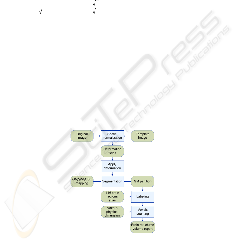
The brain anatomical structures segmentation method follows the sequence

scheme shown in Fig. 1. Spatial normalization is an image registration method [20].

The registration problem consists of optimizing the parameters q from the affine ma-

trix in order to minimize the objective function [20]. The objective function is com-

posed by the sum of squared differences between the images, as shown in Equation 1.

Some authors distinguish between different categories of alignments using the words

registration, co-registration and normalization [20]. The term normalization is usually

restricted to the inter subject registration situation, so we prefer to use the term spatial

normalization. There are two steps in the spatial normalization process: (i) estimation

of warp-field and (ii) application of warp-field with resample. The estimation of

warp-field is made using an image similarity measurement (Equation 1). In order to

perform normalization, a number of points in the template image are compared with

points in the original image. The images might be scaled differently, so a scaling

parameter denoted by s was included in the model:

[]

() ()

Mx sgx⋅−⋅

∑

(1)

where M is the affine

matrix defined by twelve parameters reproducing translation,

rotation, zoom and shearing effects [21]. The optimization algorithm used is the

Gauss-Newton based method [20]. Suppose that b

(q) is the function describing the

difference between the original and template images at voxel i, when the vector of

model parameters have values q. If the q parameters are decreased by t, Taylor’s

Theorem can be used to estimate the value of this difference:

112

() ()

()() ...

bq bq

bq t bq t t

∂

−≅ − −−

∂∂

(2)

Applying the Gauss-Newton optimization method, for iteration n, the q parameters

are updated as:

bAAAqq

TTnn

⋅⋅⋅−=

−+ 1)1(

)(

(3)

where A is the matrix of the partial derivative coefficients. The iteration is repeated

until the objective function can no longer be decreased or a maximum number of

iterations is reached. A nonlinear spatial normalization is handled for correcting gross

differences in head shapes that cannot be accounted by the affine normalization alone

Observe that the term “afine” may have different meanings. Here it means a translation of

an operator (e.g, of a square matrix). On the other hand, it is worth noticing that in the operator

theory literature an afine transformation between normed spaces is a topological isomorphism

(i.e., an invetible continuous linear transformation with a continuous inverse). A quasi afine

transformation is an injective continuous linear transformation with a dense range. If a pair of

operators are intertwined by an afine transformation, then they are said to be similar; if they are

intertwined by a quasi afine transformation, then they are says to be quasi similar (see

e.g.[21]).

.The nonlinear warps are modeled by linear combinations of smooth Discrete Cosine

Transform (DCT) basis functions, considering a tri-dimensional space, as:

)(

lililili

xdqxuxy

∑

+=+=

where l=1,2,3, q

is the j

coefficient for dimension k and d

) is the j

basis func-

tion at position x

. The d

) is defined according to:

(

)

(

)

MmIi

dandIi

KKK 2,1;

112

cos

==∀

⎟

⎠

⎞

⎜

⎝

⎛

−−

===

(4)

where d

is the mth coefficient, I is the set of voxels size. The objective function is:

()

() ()

ywgx−⋅

∑

(5)

where w is the scalar parameter, f the source image, g the template image. A linear

regularization approach based upon Bayesian framework is used in order to avoid

unnecessary deformations introducing instability. The segmentation method used an

Expectation Maximization algorithm and a Gaussian mixture modeling. It assumes

that each pixel belongs to a different class and pixel’s intensities within each class is

normal. A Bayesian model is used, where it is assumed that the modulation field U

has been drawn from a population for which the a priori probability distribution is

known. It is assumed that the prior spatial probability of each pixel is Grey Matter

(GM), White Matter (WM) or Cerebrum Spinal Fluid (CSF). The prior spatial prob-

ability images is provided by Montréal Neurological Institute (MNI) , as part of the

International Consortium of Brain Mapping (ICBM) [22]. Suppose F

is the pixel’s

intensity of the original spatial normalized image, the probability of each voxel be-

longing to each class is assigned based on Bayes rules [11].

Fig. 1. Steps of the segmentation approach.

In the next step, each pixel belonging to gray matter is labeled based on MNI ana-

tomical atlas constructed by manual segmentation, locating 116 brain structures de-

fined by Broadman’s areas [23]. Supposing the F

is the gray partition of the spatial

normalized image and assuming that it is a binary image, the brain structure is ob-

tained by logical operation as:

(, )

ijk ij ijk

G and F B

(6)

where G

ijk

is the binary image representing each of brain structure coded by k Broad-

man areas and B

ijk

is the anatomical atlas. The inverse deformation mapping is applied

to bring back the labeled structures to the original space. Each brain structure volume

is achieved by counting the pixels belonging to each Broadman area and multiplying

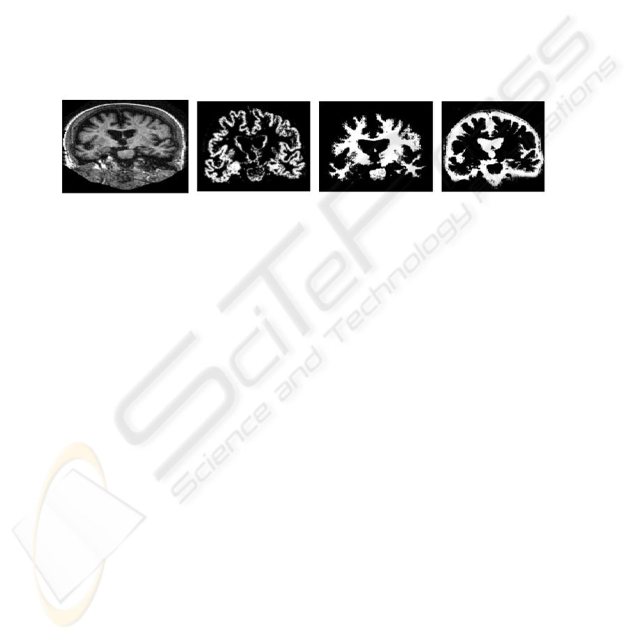
them by its physical dimensions. Figure 2 shows the 3 brain tissues (GM, WM and

CSF) segmented automatically by method described above.

Fig. 2. Brain structures segmented: (a) original MR image; (b) WM; (c) GM; and (d) CSF.

2.1 Classification

Classification is a task of machine learning and data mining areas whose solution

requires the construction of a classifier, that is, a function that assigns a class label to

instances described by a set of attributes [24]. The induction of classifiers from data

set of previous classified instances is a central problem in machine learning and data

mining researches. The classification method adopted was the naïve Bayesian classi-

fier [25]. The Bayesian classifier learns from training data the conditional probability

of each attribute A

given the class label C. Classification is done by applying Bayes

rule to compute the probability of C given the particular instance of A

, …, A

, and

then predicting the class with the highest posterior probability. The patient clinical

data set contains the brain structure volumes of each patient. These data are used as

input for the classifier training. The continuous variables, such as the brain structure

volumes, were transformed to a discrete number of intervals, reducing the number of

values and improving Bayesian classifier performance [26]. The supervised discreti-

zation method performed was the Minimum Description Length (MDL) [27]. An

attribute selection aiming to filter the most relevant attributes and to remove redun-

dant data is applied. The attributes are evaluated using correlation-based feature se-

lection (CFS) method of attribute subset selection [28] with “greedy hillclimbing” as

search method. The naïve Bayesian classifier was trained and tested on a total of 371

instances and 138 attributes. Its performance was measured performing a cross-

validation method using 10 folds [29].

3 Experiments and Text

The conducted experiments demonstrate the capability of predicting the CDR value

using patient clinical data and brain structure volume information. 371 MR T1-

weighted images from aged 18 to 96 years-old patients were used in the experiments.

Images were downloaded from the OASIS (Open Access Series Imaging Studies)

public database [30]. A number of 116 brain structures, including gray matter (GM),

white matter (WM), cerebrospinal fluid (CSF) and whole brain, were segmented

using the method described in Section 2. Patient data attributes such as age, gender,

education, socioeconomic status, and MMSE were also considered. The CDR scale

was selected as the attribute class. It was assumed a CDR scale ranging from 0 to 0.5

as normal control patient and ranging from 1 to 3 as patient in risk of dementia pa-

tient. Image processing and statistical analysis of structural T1 images were per-

formed with SPM5 (Welcome Department of Imaging Neuroscience, University Col-

lege London, visited 18/05/2008 http://www.fil.ion.ucl.ac.uk/spm). The classifier was

performed with WEKA (http://www.cs.waikato.ac.nz/ml/weka; visited at April 16

2008). Table 1 and 2 show the patient CDR description grouped by aging and gender.

Table 1. CDR considering patient ages.

Ages 0.0 0.5 1.0 2.0 Total

0 to 20 16 0 0 0 16

20 to 40 126 0 0 0 126

40 to 60 59 0 0 0 59

60 to 80 52 36 16 0 104

Over 80 33 22 10 1 66

Total 286 58 26 1 371

Table 2. CDR considering patient gender.

Gender 0.0 0.5 1.0 2.0 Total

Female 112 25 8 1 146

Male 174 33 18 0 225

Total 286 58 26 1 371

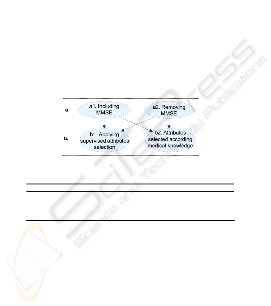
The classifier training and tests were performed according to the criteria illustrated in

Fig. 3. The criteria define the selected attributes and the set of instances following the

combinations illustrated in Fig. 3, as well. The objective is to compare the classifier

performance when using different datasets. The MMSE (Mini-Mental State Examina-

tion) is a brief questionnaire test used to assess cognition which is applied when pa-

tient has shown symptoms of cognitive deficit [18]. It is also used to predict the risk

of dementia. The MMSE score and MRI volumetric measurements can be evaluated

together, reaching a consensus diagnosis. In our experiment we performed the classi-

fier’s training with and without MMSE, because only a few patients had that informa-

tion (166 missing values). The missing MMSE scores were replaced with modes from

training data. Besides applying the supervised attribute selection method mentioned

in Section 2.1, we also considered an attribute selection set based on medical knowl-

edge. The classifier performance was measured based on sensitivity or true-positive

rate (TPR

) for each class defined according to:

FPTP

TPR

(7)

where TP

is the computing of true-positives (instances classified as class C that

belong to class C) verified in test dataset; FP

is the quantity of true-negatives is the

computing of false-positives (instances classified as C but do not belong to class C).

The classification results are summarized in Table 3, according to the selected crite-

ria. We also considered in the experiments the patients with CDR equal to 0.5, be-

cause these patients represent a very mild dementia diagnostic state, requiring usually

further information to identify a principle of cognitive deficit disorder. According to

Table 3, we noticed that the best classifier performance was achieved by using selec-

tion criterion number 1 (including MMSE score and applying supervised attributes

selection). Assuming medical knowledge, the best classifier performance was

achieved by using selection criterion number 4.

Fig. 3. Classifier training and tests strategy.

Table 3. Summarizing the results.

Selection Criteria TPR [%] 0.0³ TPR [%] >0³

1 a1 b1 90.4 96.3

2 a2 b1 88.4 96.3

3 a1 b2 89.5 88.9

4 a2 b2 86.9 92.6

The attributes selected by supervised attribute selection described in Section 2.1 are

reported in Table 4 (line 1) sorted by highest to lowest relevance. The attributes se-

lected by medical knowledge [31] are summarized in Table 4, as well. The attributes

from patient dataset are described at Marcus et al. [30]. The remainding attributes are

from automated brain structures segmentation algorithm described in Section 2, based

on brain anatomical atlas describing the Broadman areas [31].

Table 4. Attributes used: ¹ Patient data from OASIS dataset; ² Brain tissues volumes normal-

ized by total brain volume got from automated segmentation process; ³ Brain structures volume

got from automated segmentation process;

The MMSE was used only in criterion set number

N Total Attributes

1,2

MMSE¹

, nWBV¹, VLiquor², nWhite², Supp_Motor_Area_L², Cin-

gulum_Mid_L², Hippocampus_L², Hippocampus_R², ParaHippocampal_R²,

Cuneus_R², Angular_R², Caudate_L², Thalamus_L², Thamalus_R²

3,4

Gender¹, Age¹, Education¹, Socioeconomic status¹, MMSE¹

, eTIV¹, nWBV¹,

nGray², nWhite², nCSF², Cingulum_L³, Cingulum_R³, Hippocampus_L³,

Hippocampus_R³, ParaHippocampal_L³, ParaHippocampal_R³, Amyg-

dala_L³, Amygdala_R³

Evaluating the 58 subjects with CDR equal to 0.5 (questionable dementia), 69% were

classified as normal control and 31% as risk of dementia. It would be necessary to

follow those subjects up, reviewing them two or three years later, in order to predic-

tion accuracy. Fung et al [32] showed an AD patient classifier based on brain perfu-

sion marker changing observed in SPECT imaging. Their classification approach was

achieved by using SVM (support vector machines) [32].Concerning the results, they

achieved a TPR equal to 86.7% for normal control subjects and 80% for subjects with

AD. Devanand et al [33] conducted a longitudinal study performed in 139 patients

with the objective of evaluating the utility of MRI hippocampal and entorhinal cortex

atrophy in predicting conversion from mild cognitive impairment (MCI) to AD.

Based on regression models [34] in the 3-year follow-up sample, they reached 80%

specificity and 83.3% sensibility, using the attributes age, MMSE, SRT (Selective

Reminding Test) delayed recall, WAIS-R (Wechlsler Adult Intelligence Scale-

Revised), hippocampus and entorhinal cortex volumes. Fleisher et al [34] compared

volumetric MRI of whole brain and medial temporal lobe structures to clinical meas-

ures for predicting progression from MCI to AD. They obtained a 78.8% predictive

accuracy assuming hippocampus and ventricular volumes and cognitive measures,

such as MMSE, ADAS (Alzheimer’s Disease Assessment Scale), NYU recall test,

Symbol Digit Modalities Test, etc.

4 Conclusions

This paper proposed a fully automated segmentation algorithm applied to dementia

study. The paper showed also an application of a data mining method, in order to

classify patients with risk of dementia based on volumes obtained on image process-

ing. An advantage of using fully automated segmentation method should be standard-

izing brain structures volumetric assessment, allowing the patients with risk of inci-

dent AD could be followed up and treatment efficacy could be measured. As future

work, we intend to apply the method into different image sets, associated to further

clinical data, aiming to identify the risk of incidence AD in early stage.

References

1. M. Prince, "Dementia in developing countries: a consensus statement from the 10/66 De-

mentia Research Group," International Journal of Geriatric Psychiatry, vol. 15, pp. 14-20,

2000.

2. R. Nitrini, P. Caramelli, E. Herrera, V. S. Bahia, L. F. Caixeta, M. Radanovic, R. Anghi-

nah, H. Charchat-Fichman, C. S. Porto, M. T. Carthery, A. P. J. Hartmann, N. Huang, J.

Smid, E. P. Lima, L. T. Takada, and D. Y. Takahashi, "Incidence of dementia in a commu-

nity-dwelling Brazilian population," Alzheimer Dis. Ass. Disorder, vol. 18, pp. 241-246,

2004.

3. G. McKhann, D. Drachman, M. Folstein, R. Katzman, D. Price, and E. M. Stadlan, "Clini-

cal diagnosis of Alzheimer's disease: report of the NINCDS-ADRDA Workgroup under the

auspices of Department of Health and Human Services Task Force on Alzheimer's Dis-

ease," Neurology, vol. 34, pp. 939-944, 1984.

4. C. P. Hughes, L. Berg, W. L. Danziger, L. A. Coben, and R. L. Martin, "A new clinical

scale for the staging of dementia," British Journal of Psychiatry, vol. 140, pp. 566-572,

1982.

5. M. L. F. Chaves, A. L. Camozzato, C. Godinho, R. Kochhann, A. Schuh, V. L. d. Almeida,

and J. Kaye, "Validity of the clinical dementia rating scale for the detection and staging of

dementia in brazilian patients," Alzheimer Dis. Ass. Disorder, vol. 21, pp. 210-217, 2007.

6. M. B. M. M. Montaño and L. R. Ramos, "Validade da versão em português do clinical

dementia rating," Revista de Saúde Pública, vol. 39, pp. 912-917, 2005.

7. R. C. Jack, R. C. Petersen, Y. C. Xu, S. C. Waring, P. C. O'Brien, E. G. Tangalos, G. E.

Smith, R. J. Ivnik, and E. Kokmen, "Medial temporal atrophy on MRI in normal aging and

very mild Alzheimer's disease," Neurology, vol. 49, pp. 786-794, 1997.

8. C. M. d. C. Bottino, "Morphometry through magnetic imaging," Revista de Saúde Pública,

vol. 27, pp. 131-142, 2000.

9. J. Ashburner and K. J. Friston, "Voxel-based morphometry: the methods," Neuroimage,

vol. 11, pp. 805-821, 2000.

10. G. John and P. Langley, "Estimating continuous distributions in bayesian classifiers," in

Proc. Eleventh Conf. on Uncertainty in Artificial Intell., San Mateo, pp. 338-345 (1995)

11. F. L. Seixas, A. Souza, A. Plastino, D. Saade, and Aura Conci, "Clinical Dementia Rating

Score Prediction Based on Automated Brain Image Segmentation", Intern. Worksh. on

Biomedical and Health Informatics, IEEE Conference on Biomedical and Health Informat-

ics - Philadelphia, PA, November 3-5, 2008.

12. R. L. Marchetti, C. M. C. Bottino, D. Azevedo, S. K. N. Marie, and C. C. d. Castro,

"Confiabilidade de medidas volumétricas de estruturas temporais mesiais," Arquivos de

Neuro-Psiquiatria, vol. 60, 2002.

13. C. R. Jack, C. K. Twomey, A. R. Zinsmeister, F. W. Sharbrough, R. C. Petersen, and G. D.

Cascino, "Anterior temporal lobes and hippocampal formations: normative volumetric

measurements from MR images in young adults," Radiology, vol. 172, pp. 549-554, 1989.

14. C. Watson, F. Andermann, and P. Gloor, "Anatomic basis of amygdaloid and hippocampal

volume measurement by MR imaging," Neurology, vol. 42, pp. 1743-1750, 1992.

15. J. Ashburner and K. J. Friston, "Voxel-based morphometry - the methods," Neuroimage,

vol. 11, pp. 805-821, 2000.

16. C. Pennanen, C. Testa, M. P. Laakso, M. Hallikainen, E. L. Helkala, T. Hänninen, M.

Kivipelto, M. Könönen, A. Nissinen, S. Tervo, M. Vanhanen, R. Vanninen, G. B. Frisoni,

and H. Soininen, "A voxel based morphometry study on mild cognitive impairment," Jour-

nal of Neurology, Neurosurgery Psychiatry, vol. 76, pp. 11-14, 2005.

17. B. H. Ridha, V. M. Anderson, J. Barnes, R. G. Boyes, S. L. Price, M. N. Rossor, J. L.

Whitwell, L. Jenkins, R. S. Black, M. Grundman, and N. C. Fox, "Volumetric MRI and

cognitive measures in Alzheimer disease," Journal of Neurology, vol. 255, pp. 567-574,

2008.

18. M. F. Folstein, S. E. Folstein, and P. R. Hugh, "Mini-mental state: a practical method for

grading the cognitive state of patients for the clinician," Psychiatry Research, vol. 12, pp.

189-198, 1975.

19. C. R. Jack, M. M. Shiung, J. L. Gunter, P. C. O'Brien, S. D. Weigand, D. S. Knopman, B.

F. Boeve, R. J. Ivnik, G. E. Smith, R. H. Cha, E. G. Tangalos, and R. C. Petersen, "Com-

parison of different MRI brain atrophy rate measures with clinical disease progression in

AD," Neurology, vol. 62, pp. 591-600, 2004.

20. D. L. G. Hill, P. G. Batchelor, M. Holden, and D. J. Hawkes, "Medical image registration,"

Physics in Medicine and Biology, vol. 46, pp. 1-45, 2001.

21. C. S. Kubrusly, Invariant subspaces and quasiaffine transforms of unitary operators, Pro-

gress in Nonlinear Differential Equations and their Applications, vol.42, pp.167--173,

2000.

22. A. C. Evans, D. L. Collins, S. R. Mills, E. D. Brown, R. L. Kelly, and T. M. Peters, "3D

statistical neuroanatomical models from 305 MRI volumes," Proceedings IEEE-Nuclear

Science Symposium and Medical Imaging Conference, pp. 1813-1817, 1993.

23. Y. Alemán-Gómez, L. Melie-García, and P. Valdés-Hernandez, "IBASPM: toolbox for

automatic parcellation of brain structures," Neuroimage, vol. 27, 2006.

24. N. Friedman, D. Geiger, and M. Goldszmidt, "Bayesian network classifiers," Machine

Learning, vol. 29, pp. 131-163, 1997.

25. R. O. Duda , P. E. Hart and D. G. Stork, Pattern classification. 2nd Ed. New York: John

Wiley & Sons, 2001.

26. R. Abraham, B. Simha, and S. S. Ivengar, "A comparative analysis of discretization meth-

ods for medical datamining with Näive Bayesian classifier," in International Conference on

Information Technology, pp. 235-236, 2006.

27. U. M. Fayyad and K. B. Irani, "Multi-interval discretization of continuous-valued attributes

for classification learning," in Proceedings Thirteenth International Joint Conference on

Artificial Intelligence, San Francisco, pp. 1022-1027, 1993.

28. M. A. Hall, "Correlation-based feature selection for machine learning," in Philosophy. vol.

Doctor: University of Waikato, 1999.

29. J. Han and M. Kamber, Data mining: concepts and techniques, Morgan Kaufman, 2006.

30. D. S. Marcus, T. H. Wang, J. Parker, J. G. Csernansky, J. C. Morris, and R. L. Buckner,

"Open access series of imaging studies (OASIS): cross-sectional MRI data in young, mid-

dle aged, nondemented and demented older adults," Journal of Cognitive Neuroscience,

vol. 19, pp. 1498-1507, 2007.

31. A. S. d. Souza, "Espectroscopia de prótons na demência de Alzheimer e no

comprometimento cognitivo," in Faculdade de Medicina. vol. Doctor: Universidade de São

Paulo, (2005).

32. G. Fung and J. Stoeckel, "SVM feature selection for classification of SPECT images of

Alzheimer's disease using spatial information," Knowledge and Information Systems, vol.

11, pp. 243-258, 2007.

33. D. P. Devanand, G. Pradhaban, X. Liu, A. Khandji, S. Santi, S. Segal, H. Rusinek, G. H.

Pelton, L. S. Honig, R. Mayeux, Y. Stern, M. H. Tabert, and M. J. Leon, "Hippocampal

and entorhinal atrophy in mild cognitive impairment," Neurology, vol. 68, pp. 828-836,

2007.

34. A. S. Fleisher, S. Sun, C. Taylor, C. P. Ward, A. C. Gamst, R. C. Petersen, C. R. Jack, P. S.

Aisen, and L. J. Thal, "Volumetric MRI vs clinical predictors of Alzheimer disease in mild

cognitive impairment," Neurology, vol. 70, pp. 191-199, 2008