
Empirical Descriptors Evaluation for Mass Malignity
Recognition
Imene Cheikhrouhou
1,2
, Khalifa Djemal
1
, Dorra Sellami Masmoudi
2
Hichem Maaref
1
and Nabil Derbel
2
1
University of Evry Val dEssonne (UEVE), France
2
National Engineering school of Sfax (ENIS), BP W, 3038 Sfax, Tunisia
Abstract. In breast cancer field, radiologists and researchers aim to discriminate
between masses due to benign breast diseases and tumors due to breast cancer.
In general, benign masses have circumscribed contours, whereas, malignant tu-
mors appear with spiculated and irregular boundaries. Recently, we proposed an
original mass description based on three morphological mass descriptors, which
are SPICULation (SPICUL), Contour Derivative Variation (CDV) and Skeleton
End Points (SEP). In this paper, we detail an empirical mass evaluation based
on these morphological descriptors which intend to distinguish between malig-
nant and benign lesions. This evaluation is, first, assured by following descriptors
evolution in two independent data sets: Alberta and MIAS. Secondly, for these
two data sets, the Receiver Operating Characteristics (ROC) analysis is applied.
A comparison between the classic use of Area (A) and Perimeter (P) descriptors
only, and a combination with our three original evaluated descriptors is done. Ob-
tained results proves that classification accuracy of the descriptors combination
including: SPICUL, SEP, CDV, A and P outperforms that of the classic descrip-
tors: A and P. Indeed, our original mass description provides the best Area un-
der ROC A
z
= 0.986 for Alberta data set and A
z
= 0.9792 for the MIAS data
set. Therefore, we affirm that our three original descriptors can serve as good
shape descriptors for the benign-versus-malignant classification of breast masses
on mammograms.
1 Introduction
Breast cancer is one of the most common diseases that threaten woman life and sci-
entific studies have shown that the mortality rate caused by breast cancer is decreased
by early detection and treatment. Mammography is known to be the most effective
screening method and is credited with reducing breast cancer mortality by at least 30%.
However, screening mammography program requires a large number of radiologists
with special training in this field which could involve problems such as high costs and
visual fatigue. For this reason, several researches aim to develop Computer Aided Diag-
nosis systems (CAD) that could automatically analyze mammographic images [1], [2],
[3]. These CAD systems focus on detection, description and classification of breast ab-
normalities which could be either a mass or a microcalcification, or sometimes both
Cheikhrouhou I., Djemal K., Sellami Masmoudi D., Maaref H. and Derbel N. (2009).
Empirical Descriptors Evaluation for Mass Malignity Recognition.
In Proceedings of the 1st International Workshop on Medical Image Analysis and Description for Diagnosis Systems, pages 91-100
DOI: 10.5220/0001815400910100
Copyright
c
SciTePress

[4] [5]. Breast Imaging Reporting and Data System (BIRADS) standard is a mam-
mographic lexicon developed by American College of Radiology (ACR) [6] for the
mammographic lesions description. This lexicon includes descriptors such as the mass
margins and the microcalcification distribution that defines final assessment categories
and suspicion level of mammographic abnormalities.
According to BIRADS, masses classification depends on contour complexity. The
descriptors used to define masses are shape and margin [6]. A benign mass is a regular
form, generally round or oval with a well circumscribed boundary, whereas a typical
malignant tumor is an irregular, spiculated form with a rough boundary. There could be
also, some unusual cases which cause difficulties in pattern classification studies [17].
Many works focus on mass classification with contour descriptors. A study by Chen, et
al [1] reported 0.982 as the best area under the receiver operating characteristic (ROC)
curve (A
z
) when using five new morphological features that concretize variations in
boundary delineation. Guo et al [20] computed the fractal dimension to characterize the
complexity of breast mass contour. Rangayyan and Nguyen [19] presented a study of
fractal dimension including the ruler method and the box counting method that leads to
A
z
= 0.89 and a study of fractional concavity that provides A
z
= 0.88. Their combi-
nation yielded the highest area under the ROC curve of 0.93. Some studies focus on the
evaluation of existing descriptors because of its significant importance in downstream
treatments and final decision. This evaluation is in order to preserve pertinent descrip-
tors and to propose improvements for the others. We have proposed microcalcification
evaluation that brings to improve the rectangularity formulation [15] and hence, the
classification accuracy.
We have proposed previously [14] three pertinent descriptors which could describe
mass forms and that could be very useful in CAD systems. So, to prove their perfor-
mance, mammographic images are first preprocessed to obtain filtered [21] and seg-
mented [22] [16][13][18] masses to could focus on detailing a descriptor evaluation for
mass malignity recognition by means of two data sets Alberta and MIAS which repre-
sent variety of cases. Our main objective in this evaluation is to prove how descriptors
react towards complexity contour. The paper is organized in four sections. Next sec-
tion is preserved to the evaluation of the morphological descriptors: SPICUL, CDV and
SEP applied to two different data sets Alberta and MIAS. Section 3 shows experimen-
tal results. ROC curves associated to both data sets are represented to validate features
ability to discriminate between benign masses and malignant tumors. We present also,
a comparison with other methods that characterize shape complexity in the same data
sets. Finally, we conclude in section 4.
2 Descriptors Evaluation through Two Mammographic Data Sets
Evaluated morphological descriptors are Contour Derivative Variation (CDV), Spicula-
tion (SPICUL) and Skeleton End Points (SEP) [14]. Selected descriptors for validation
are evaluated through two data sets. The first data set B1 was obtained from Screen
Test: the Alberta Program for the Early Detection of Breast Cancer [7] [8]. From this
data set, we exploit 35 benign masses, most of which are circumscribed, and 35 malig-
nant tumors, most of which are spiculated, as typically encountered in mammographic
92
images. The second data set named B2 is from the Mammographic Image Analysis
Society (MIAS) database [9]. From which we use 28 benign masses and 28 malignant
ones including circumscribed and spiculated cases in both benign and malignant cate-
gories. Spiculated benign masses and circumscribed malignant tumors are unusual, and
tend to cause difficulties in pattern classification studies.
2.1 Contour Derivative Variation (CDV)
0 50 100 150 200 250 300 350 400 450
−1
−0.8
−0.6
−0.4
−0.2
0
0.2
0.4
0.6
0.8
1
0 50 100 150 200 250 300 350 400
−1
−0.8
−0.6
−0.4
−0.2
0
0.2
0.4
0.6
0.8
1
0 50 100 150 200 250 300 350 400 450
−1
−0.8
−0.6
−0.4
−0.2
0
0.2
0.4
0.6
0.8
1
0 50 100 150 200 250 300 350 400 450
−1
−0.8
−0.6
−0.4
−0.2
0
0.2
0.4
0.6
0.8
1
0 50 100 150 200 250 300 350 400
−1
−0.8
−0.6
−0.4
−0.2
0
0.2
0.4
0.6
0.8
1
0 50 100 150 200 250 300 350 400
−1
−0.8
−0.6
−0.4
−0.2
0
0.2
0.4
0.6
0.8
1
0 200 400 600 800 1000 1200
−1
−0.8
−0.6
−0.4
−0.2
0
0.2
0.4
0.6
0.8
1
0 100 200 300 400 500 600 700 800 900
−1
−0.8
−0.6
−0.4
−0.2
0
0.2
0.4
0.6
0.8
1
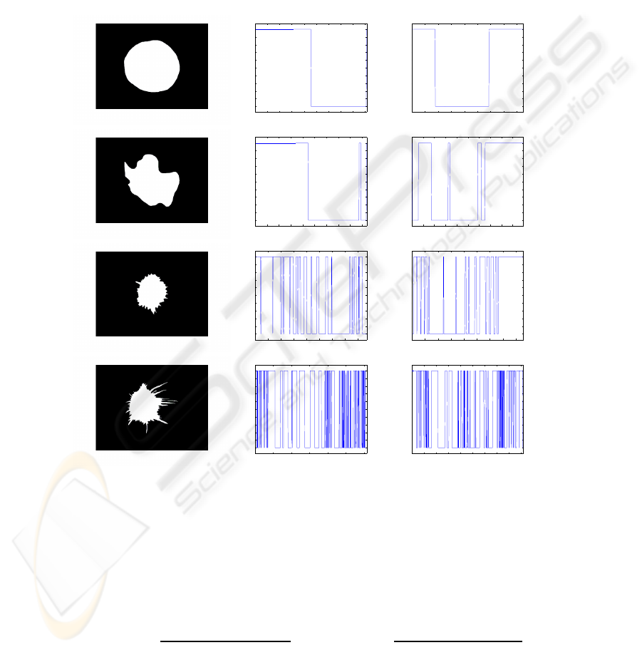
a) b) c)
Fig.1. Contour Derivative Variation related to X and Y: a) Original images, b) CDVX and c)
CDVY.
As given in [14], for the k
th
contour point with coordinates X(k) and Y (k), we
define the Contour Derivative related to x-coordinate (CDX) and Contour Derivative
related to y-coordinate (CDY) as follows:
CDX(k) =
X(k + 1) − X(k − 1)
2
CDY (k) =
Y (k + 1) − Y (k − 1)
2
(1)
93
where X(k + 1) and Y (k + 1) are the (k + 1)
th
contour point coordinates, respectively,
X(k − 1) and Y (k − 1) are the (k − 1)
th
contour point coordinates.
We note CDVX (resp. CDVY) the number of CDX (resp. CDY) variation sign from
positiveto negativeor from negativeto positive values. So, Contour DerivativeVariation
(CDV) is the CDVX and CDVY total sum.
Figure 1 shows images from the two data sets B1 and B2 ordered from benign to
malignant. Subjectively, we can note that for regular masses we should have CDVX=2
and CDVY=2 as shown in fig.1, in the first image with circular shape which provides
CDV=4. The second which is lobulated has low CDV value (CDV=12). The last two
images which are irregular and spiculated, have more sign variations in contour deriva-
tive. Especially for high spiculated masses as the forth
th
example, CDVX reaches 92
and CDVY reaches 88 which provides a high CDV value (CDV=180). We can notice
that CDV will increase considerably when contour becomes more and more complex.
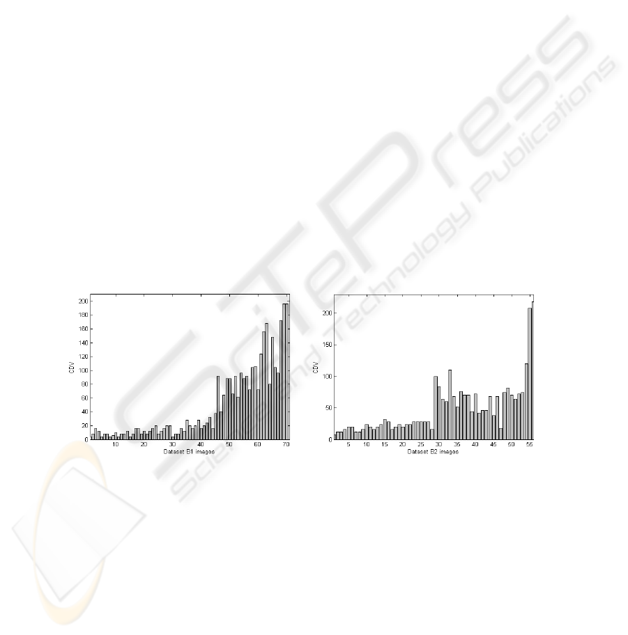
To objectively prove this observation, we plot CDV values for both data set B1 and
data set B2. Figure.2 a) shows all data set B1 images: from image n
o
1 to n
o
35, we
present benign images and from image n
o
36 to n
o
70, we present malignant ones. Also,
figure.2 b) shows all data set B2 images: from image n
o
1 to n
o
28, we present benign
images and from image n
o
29 to n
o
56, we present malignant ones. We will preserve
this distribution for all next evaluations. For data set B1, benign masses still under the
value CDV=30 and malignant ones are higher than CDV=30 except of 7 images. For
the second data set B2, benign images are all under CDV=30 and for malignant cases,
all images exceed this value except image n
o
47 with CDV=18. These results prove that
this descriptor has the ability to distinguish between benign and malignant masses for
the two data sets B1 and B2.
a) b)
Fig.2. CDV evaluation for: a) data set B1 and b) data set B2.
2.2 Spiculation (SPICUL)
In [14], we propose a new feature named spiculation (SPICUL) defined as follows:
S =
X
k
SpiculX(k) +
X
k
SpiculY (k) (2)
94
where k represents the k
th
contour point, SpiculX(k) (respectively SpiculY (k)) is the
number of points having the same x-coordinate (resp. the same y-coordinate).
Masses from the two data sets, represented in fig.1 are reproduced in the same order
of increasing malignity to be evaluated with the SPICUL descriptor. Results are given
in Table 1 which shows that when the mass is more spiculated, (SPICUL) increases
successively from 0.3967 to 6.0081.
Table 1. SPICUL value for six masses ordered from benign to malignant.
Mass 1 Mass 2 Mass 3 Mass 4
SPICUL 0.3967 0.6130 1.2514 6.0081
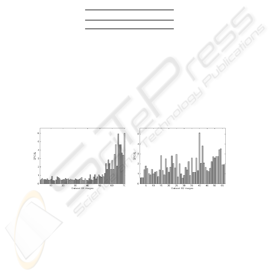
For evaluating the whole images, we show in fig.3 evaluation of the descriptor
SPICUL. Data set B1 represented in fig.3 a) indicates that the first 35 benign images
have nearly similar values which are all strictly under SPICUL=1. Otherwise, all be-
nign masses are identified correctly. For malignant images, the majority of masses are
well recognized and are well separated from benign masses with values between 2 and
6. But, 14 malignant cases are considered benign also. Data set B2 in fig.3 b) shows
that SPICUL makes many errors in benign case recognition. So, SPICUL evaluation in
data set B1 proves its strength to discriminate between malignant and benign images.
And SPICUL evaluation, in data set B2, proves that errors are caused essentially by the
presence of irregular forms in benign class that have higher SPICUL values.
a) b)
Fig.3. SPICUL evaluation for: a) data set B1 and b) data set B2.
2.3 Skeleton End Points (SEP)
Skeleton provides a simplified version of the object at one pixel width. This represen-
tation makes easy complex images processing such as digital fingerprint, handwritten
letters and [10] blood vessels images . In mammographic field, and especially when we
treat complexity contour, skeleton seems to be very useful. In fact, for regular shapes,
skeleton has few branches, and for irregular contours, skeleton becomes more complex
95
and has several ramifications. In [1] authors study skeleton concept in breast sonogram
images by computing the number of skeleton points. This entity is very sensitive to
lesion size. To avoid this constraint, we developed in [14] a new skeleton formulation
adapted to our objectives,based on skeleton branches number by computing the number
of skeleton End Points (SEP).
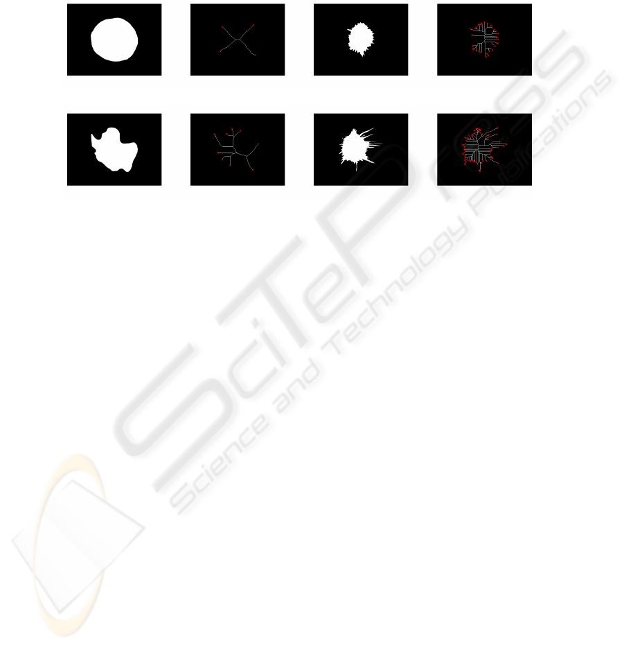
a) c)
b) d)
Fig.4. Skeletonization: Four masses and relative skeletons with their end points (SEP).
As a first SEP evaluation, we plot in fig.4 skeletons and skeleton end points for the
same masses studied in fig.1 and Table 1 extracted from B1 and B2. Fig.4 a) which is
a regular circle have SEP=4. For the lobulated form b) SEP raises slightly with succes-
sively 7 ramifications. Irregular forms, (such as c and d) have skeletons more compli-
cated and also have the higher SEP values such as the last mass d) with SEP=55. This
first observation confirms the descriptor performance in distinguishing between regular
and irregular masses, then between benign and malignant cases.
As a second SEP evaluation, we test SEP evolution across the two data sets in fig.5.
We notice that, for fig.5 a), for the data set B1, benign masses could be visually dis-
tinguished with their low values under 13. However, for malignant masses, SEP highly
increases with values that overpass SEP=50. The gap between SEP values favors dis-
crimination between the two classes. For the data set B2, fig.5 b), benign forms are all
recognized correctly ( all SEP values are ≤ 13). But, in malignant forms, the skeleton
have some errors. It confounds some benign and malignant cases.
It should be noted that, for all evaluation examples, data set B1 recognizes better be-
nign and malignant classes. And as we have said before, data set MIAS have some spic-
ulated forms in benign class and some circumscribed forms in malignant class which
clarify why this data set has less discrimination between the two classes. For this rea-
son, we notice that descriptors for data set B2 translate well their information about
complexity contour which explain that we find low descriptor values in malignant cases
and high descriptor values in benign cases.
96
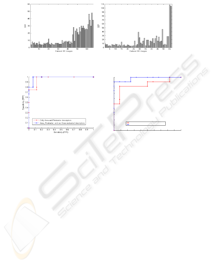
a) b)
Fig.5. SEP evaluation for: a) data set B1 and b) data set B2.
0 0.1 0.2 0.3 0.4 0.5 0.6 0.7 0.8 0.9 1
0
0.1
0.2
0.3
0.4
0.5
0.6
0.7
0.8
0.9
1
Sensitivity (FPF)
Specificity (TPF)
Only Area and Perimeter descriptors
Area, Perimeter, and our three evaluated descriptors
a) b)
Fig.6. ROC curve associated to: a) data set B1 and b) data set B2.
3 Experimental Results
Since mass classification depends on mass size, we compute mass area (A) which is,
in digital images, given by the number of pixels that belong to the mass. As a sec-
ond geometrical feature, we add perimeter which can be easily obtained by computing
boundary pixels [11]. These geometrical descriptors generally ameliorate classification
rate. First, in this section, we use evaluated descriptors: CDV, SPICUL and SEP for
classification through SVM classifier, joined to informative descriptors Area (A) and
Perimeter (P). To evaluate the classification performance, we use the so-called Receiver
Operating Characteristic (ROC) analysis, which is now used routinely for many clas-
sification tasks. A ROC curve is a plot of the classification sensitivity (TPF) as the
ordinate versus the specificity (FPF) as the abscissa. For a given classifier, ROC curve
is obtained by continuously varying the threshold associated with its decision function.
At any given FPF, a ROC curve with a higher TPF corresponds to a better classification
performance. The overall classification accuracy is summarized by the area under the
ROC curve (A
z
).
In this section, we classify data set B1 and B2, first with all cited descriptors: Con-
tour Derivative Variation (CDV), Spiculation (SPICUL), Skeleton end points (SEP),
97

Perimeter (P) and Area (A) (5 descriptors), and secondly with only P and A (2 descrip-
tors) in order to keep a comparison between our proposed descriptors and known ones.
These descriptors are used as entries to SVM classifier which seems to be an excellent
candidate for several classification tasks such as medical applications [12].
Fig.6 a) shows ROC curve of data set B1 in both cases 5 descriptors and 2 de-
scriptors. We notice that, although ROC curve of (5 descriptors) outperforms that of
(2 descritors), for both cases, TPF fraction still very high for FPF values. This proves
the pertinence of descriptors adopted even for malignant images with similar aspect to
benign ones and contrarily. Area under ROC computed for 5 descriptors is A
z
= 0.986
and for 2 descriptors is A
z
= 0.97 as given in Table 2.
Fig.6 b) represents ROC curve of data set B2 in both cases 5 descriptors and 2 de-
scriptors. This data set contains circumscribed and spiculated masses in both malignant
and benign cases. Although this new organization makes classification task very diffi-
cult, the area under ROC preserves a high value of A
z
= 0.9792 especially in the case
of 5descriptors. For two descriptors, classification accuracy decreases significantly and
provides A
z
= 0.854 as shows in Table 2.
Table 2. Area under ROC for the two data sets.
A
z
Area and Perimeter Area, Perimeter, SPICUL, CDV, and SEP
B1 0.97 0.986
B2 0.854 0.9792
We provide a final evaluation based on a comparison with a recent work. Rangayyan
and Nguyen [19] focused on contour description on mammograms and detailed four
methods to compute the fractal dimension of the contours of breast masses, including
the ruler method and the box counting method applied to 1D and 2D representations
of the contours. The methods were applied to the same data sets that we exploit: the
Alberta [7] and MIAS [9] data sets. Receiver operating characteristics (ROC) analysis
was performed to assess and compare the performance of fractal dimension methods
and the use of the five descriptors: SPICUL, SEP, CDV, P and A in the classification of
breast masses as benign or malignant. This comparison is presented in Table 3.
Table 3. Area under ROC for the two data sets in the case of fractal dimension and our descriptors.
A
z
Data set B1 Data Set B2
1D ruler 0.91 0.8
2D ruler 0.94 0.81
1D box counting 0.89 0.8
2D box counting 0.9 0.75
our descriptors 0.986 0.9792
We notice that, for the use of fractal dimension or our descriptors, data set B1 pro-
vides usually better results in classification than data set B2 because of the existence
98

of atypical masses (slightly lobulated or spiculated benign masses and round or cir-
cumscribed malignant tumors) which cause more misclassified cases than the data set
B1. Also, the combination of the five descriptors: SPICUL, SEP, CDV, P and A outper-
forms the use of fractal dimension, that provides as better results with the use of 1D
ruler method A
z
= 0.94 for data set B1 versus A
z
= 0.986 in our case and A
z
= 0.81
for data set B2 versus A
z
= 0.9792.
4 Conclusions
In this paper, we propose an empirical evaluation of three morphological descriptors
which are useful in the analysis of breast masses contours. For evaluation, we use two
independent data sets from Alberta and MIAS. These data sets are widely different and
independent which allows as to generalize from final results. When computing descrip-
tors, we notice their ability to capture diagnostically important details of shape related to
spicules and lobulations. The proposed descriptors, joined to the geometrical features
perimeter and area, have provided high classification accuracies when discriminating
between benign breast masses and malignant tumors. This result outperforms classifi-
cation accuracy of the two descriptors P and A for the two data sets, which prove the
performance and the precision of these descriptors. In future works, we intend to eval-
uate the performance of each descriptor apart and to compare them to other pertinent
descriptors cited in literature which have proven a high performance in mass classifi-
cation. Also, we intend to modify classification tools in order to reduce False Positive
Fraction and to further maximize True Positive fraction.
References
1. C-M Chen, Y-H Chou, K-C Han, G-S Hung, C-M Tiu, H-J Chiou, S-Y Chiou, ”Breast Le-
sions on Sonograms: Computer-aided Diagnosis with Nearly Setting-Independent Features
and Artificial Neural Networks”, Radiology, Fvrier 2003, p504-514.
2. H-K Chiang, C-M Tiu, G-S Hung, S-C Wu, T-Y Chang, Y-H Chou, ”Stepwise Logistic Re-
gression Analysis of Tumor Contour Features for Breast Ultrasound Diagnosis”, IEEE Ul-
trasonic Symposium, 2001, p1303-1306
3. D-R Chena, R-F Changb, C-J Chenb, M-F Hob, S-J Kuoa, S-T Chena, S-J Hungc, W-K
Moond, ”Classification of breast ultrasound images using fractal feature”, Elseiver, Journal
of Clinical Imaging Vol, 29, 2005, p 235-245
4. S Kim and S Yoon, ”Bi-rads features-based computer-aided diagnosis of abnormalities in
mammographic images”. In 6th International Special Topic Conference on ITAB,(2007).
5. A Oliver, J Freixenet, R Marti, J Pont, E Prez, E-R-E. Denton and R Zwiggelaar, ”A
Novel Breast Tissue Density Classification Methodology”, IEEE Transactions On Informa-
tion Technology In Biomedicine, Vol. 12, No. 1, January 2008, p55-65.
6. American College of Radiology ”BI-RADS (Breast Imaging Reporting and Data System”)
Frensh Edition realized by SFR (Societe Francaise de Radiologie), Third Edition, 2003.
7. Alberta Program for the Early Detection of Breast Cancer. Alberta Cancer Board, 2001.
8. H Rangayyan, R., and J Desautels, ”Content-based retrieval and analysis of mammographic
masses”. In Journal of Electronic Imaging.(2005).
9. The mammographic image analysis society digital mammogram database. In
http://www.wiau.man.ac.uk/services/MIAS/MIASweb.html.
99

10. S Lam, Y., and Y Hong, ”Blood vessel extraction based on mumford shah model and skele-
tonization”. In Proceedings of the Fifth International Conference on Machine Learning and
Cybernetics.(2006) Press.
11. B Jahne, ”Digital image processing : concepts, algorithms, and scientific applications”
(1993). In Springer-Verlag.
12. L Wei, Y Yang, R M. Nishikawa, and Yu Jiang ”A Study on Several Machine-Learning
Methods for Classification of Malignant and Benign Clustered Microcalcifications”, IEEE
Transactions On Medical Imaging, Vol. 24, NO. 3, March 2005, p371-380
13. K Djemal, W Puech and B Rossetto. Active Contours Propagation in a Medical Images
Sequence With a Local Estimation, European Signal Processing Conference. EUSIPCO’02,
Volume 1, pp: 41-44, September 2002, Toulouse, France.
14. I Cheikhrouhou, K Djemal, D Sellami, N Derbel and H Maaref ”New mass description in
mammographies”. 1st International Workshops on Image Processing Theory, Tools & Ap-
plications, IPTA’08, Sousse, Tunisia, 24-26 November 2008.
15. I Cheikhrouhou, K Djemal, D Sellami Masmoudi, N Derbel and H Maaref. Abnormalities
description for breast cancer recognition. Intenational Conference on E-Medical Systems,
Morroco, 2007, p198-205.
16. K Djemal, W Puech and B Rossetto. Automatic Active Contours Propagation in a Sequence
of Medical Images. International Journal of Images and Graphics. vol.6 , n. 2, pp :267-292 ,
2006.
17. NR Mudigonda, RM Rangayyan, JEL Desautels: ”Gradient and texture analysis for the clas-
sification of mammographic masses”. IEEE Trans Med Imag 2000, p1032-1043.
18. K Djemal, F Bouchara and B Rossetto. Image Modeling and Regionbased Active Contours
Segmentation. Int. Conf. Vision, Modeling and Visualization VMV’02, ISBN:3-89838-034-
3, pp: 363-370, Novembre 2002, Erlangen, Germany.
19. R-M. Rangayyan and T-M. Nguyen ”Fractal Analysis of Contours of Breast Masses in Mam-
mograms”, Journal of Digital Imaging, Vol 20, No 3, 2007, p223-237.
20. Q Guo, V Ruiz, J Shao, F Guo ”A novel approach to mass abnormality detection in mam-
mographic images”, In Proceedings of the IASTED International Conference on Biomedical
Engineering, Innsbruck, Austria, 2005, p180-185.
21. K Djemal. Speckle reduction in ultrasound images by minimization of total Variation. IEEE
International Conference on Image Processing (ICIP), Volume 3, ISBN: 0-7803-9134-9, pp:
357-360, September 2005, Genova, Italya.
22. K Djemal, W Puech and B Rossetto. Geometric Active Contour Model Using Level Set
Methods For Objects Tracking In Images Sequence. International Conference on Sciences
of Electronics, Technology of Information and Telecommunication, SETIT’04, Mars 2004,
Sousse, Tunisia.
100
