
3D OBJECT RECONSTRUCTION FROM SWISSRANGER SENSOR
DATA USING A SPRING-MASS MODEL
Babette Dellen
1,2
, Guillem Aleny`a
2
, Sergi Foix
2
and Carme Torras
2
1
Bernstein Center for Computational Neuroscience, Max-Planck Institute for Dynamics and Self-Organization
Bunsenstrasse 10, G¨ottingen, Germany
2
Institut de Rob`otica i Inform`atica Industrial (CSIC-UPC), Llorens i Artigas 4-6, 08028 Barcelona, Spain
Keywords:
Swissranger sensor, 3D reconstruction, Spring-mass model.
Abstract:
We register close-range depth images of objects using a Swissranger sensor and apply a spring-mass model for
3D object reconstruction. The Swissranger sensor delivers depth images in real time which have, compared
with other types of sensors, such as laser scanners, a lower resolution and are afflicted with larger uncer-
tainties. To reduce noise and remove outliers in the data, we treat the point cloud as a system of interacting
masses connected via elastic forces. We investigate two models, one with and one without a surface-topology
preserving interaction strength. The algorithm is applied to synthetic and real Swissranger sensor data, demon-
strating the feasibility of the approach. This method represents a preliminary step before fitting higher-level
surface descriptors to the data, which will be required to define object-action complexes (OACS) for robot
applications.
1 INTRODUCTION
The automatic reconstruction and model building of
complex physical objects is important to guide robotic
tasks such as grasping and view-point changes, and
more in general to predict the outcome of robot ma-
nipulations. Due to improvements during the last
decade in the field of 3D time-of-flight sensors (TOF),
faster and more accurate data can now be obtained
from these sensors. The Swissranger sensor provides
an excellent tool for 3D robot exploration tasks. The
camera can be mounted on a robot arm, depth images
can be acquired in real time, and objects can be si-
multaneously manipulated and reconstructed. The re-
sulting depth images in this specific application are of
low resolution and contain large uncertainties, requir-
ing the adaptation and development of suitable mod-
els.
Previously, several methods have been proposed
to reconstruct 3D object surfaces from a cloud of
3D data points, e.g. dynamic particles [Szeliski
et al., 1992], implicit-surface based methods [Hoppe
et al., 1992], volumetric methods [Curless and
Levoy, 1996], tensor-voting based methods [Tang and
Medioni, 2002], Voronoi-based surface reconstruc-
tion [Amenta et al., 1998], level sets [Zhao et al.,
2000], and surface fitting with radial basis functions
[Carr et al., 2001]. Techniques based on dynamic par-
ticles [Szeliski et al., 1992] have the advantage that a
microscopic model of the object is constructed, which
can be used to model outcome of robot action applied
to deformable objects, e.g. the manipulation of a ta-
ble cloth [Cuen et al., 2008]. In this paper, we propose
a method based on a system of elastically interacting
masses. The proposed model differs from previous
approches based on dynamic particles in the way the
data is incorporated into the model and in the spe-
cific choices of the interaction functions. A novel fea-
ture of this algorithm is the inclusion of a damping
and a noise term which drive the system towards a lo-
cal minimum, an idea similar to simulated annealing.
The model constitutes a preliminary step before fitting
higher-level surface descriptors to the data. These en-
tities will then provide a solid basis for guiding ob-
ject actions, i.e. viewpoint changes and actions of the
robot gripper.
The reconstruction process consists of the follow-
ing steps: Image capture (a), coarse registration (b),
fine registration (c), and implicit surface modeling via
a spring-mass model (d), which is introduced in Sec-
tion 2. Steps a-c are described in Section 3.
368
Alenya G., Foix S., Torras C. and Dellen B. (2009).
3D OBJECT RECONSTRUCTION FROM SWISSRANGER SENSOR DATA USING A SPRING-MASS MODEL.
In Proceedings of the Fourth International Conference on Computer Vision Theory and Applications, pages 368-372
DOI: 10.5220/0001819603680372
Copyright
c
SciTePress
2 THE MODEL SYSTEM
The basic framework we consider can be defined as
follows. Let P be a set of data points with measured
position X
p
= (X
p
,Y
p
,Z
p
) in a three-dimensional
space. To each data point, we assign a mass
point defined by a continuous position variable x
p
=
(x
p
,y
p
,z
p
) and a velocity variable v
p
= (u
p
,v
p
,w
p
).
The masses are moving under the influence of a
data force
F
data
= k(X
p
− x
p
) , (1)
where k is a parameter.
Each mass q exerts a force
F
int
(p,q) = κ(p, q)(x
q
− x
p
) , (2)
on p, if q is in the neighborhood N(p) of p.
We consider two different models, A and B. In
model A, κ(p,q) is equal to a constant c, while in
model B the function κ(p, q) depends on the angle
between the surface normal of particle q and the dif-
ference vector x
p
− x
q
, such that
κ(p, q) = 2c[π/2 − θ(x
p
− x
q
,n
q
)]/π , (3)
where n
q
is the surface normal at q and
θ(a,b) =
(
∠(a,b) if ∠(a,b) ≦ π/2,
π− ∠(a,b) if ∠(a,b) > π/2.
(4)
Note that ∠(a,b) is the inner angle enclosed by a and
b and thus does not grow larger than π. Eq. 4 ensures
that the interaction force depends only on the orienta-
tion of the surface normal relative to the mass.
A schematic comparison of model A and B is pro-
vided in Fig. 1. While the interaction forces in model
A only depend on the relative distances of neighbor-
ing particles, model B takes into account the position
of a particle with respect to the surface orientation
of the neighboring particles. This has the advantage
that the data is preferably smoothed in the direction
of the local surface normal, thus reducing undesired
contractions of the object model and oversmoothing
at edge discontinuities.
The dynamics of the system is described by a sys-
tem of coupled ordinary differential equations
dx
p
/dt = v
p
(5)
dv
p
/dt = F
data
+ F
int
+ τ− γv
p
, (6)
where τ is a noise term and γv
p
a damping term with
damping constant γ. These additional forces have
been added to move the dynamical system towards a
local minimum.
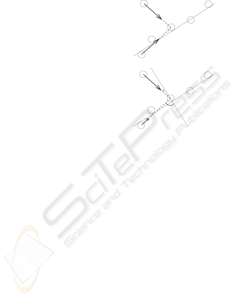
(a) Model A
(b) Model B
Figure 1: Schematic of particle interaction models. (a) In
model A, the interaction forces (thick arrow) are indepen-
dent of the orientation of the local surface (thin line). (b) In
model B, the interaction forces are stronger in the direction
of the local surface normal
2.1 Finding a Local Minimum
The system of differential equations is solved using a
4th order Runge Kutta technique with a step size of
0.1, starting from random initial conditions. Cooling
is introduced through the damping force and the noise
term τ. With the course of time, we decrease the noise
according to
τ = p
r
(n
i
− t)/n
i
(7)
where n
i
is the total number of iterations and t is the
current iteration number. The number p
r
is drawn
from a Gaussian distribution with a standard devia-
tion of 5 pixels.
2.2 Surface Normals
Following Liang and Todhunter [Liang and Tod-
hunter, 1990], we define the local covariance matrix
at p as
C =
∑
q∈N
s
(p)
(x
q
− x
m
) · (x
q
− x
m
)
T
/n , (8)
where n is the number of points in the local neighbor-
hood N
s
(p) of p, and
x
m
=
∑
q∈N
s
(p)
x
q
/n (9)
3D OBJECT RECONSTRUCTION FROM SWISSRANGER SENSOR DATA USING A SPRING-MASS MODEL
369
is the mean position vector. The local plane which
minimizes, in the least squares sense, the orthogo-
nal projections of all points in N
s
(p) onto the plane
is given by the two eigenvectors corresponding to the
two largest eigenvalues.
−25 −20 −15 −10 −5 0 5 10 15 20 25
−25
−20
−15
−10
−5
0
5
10
15
20
25
(a) Data view 1
−30 −20 −10 0 10 20 30−20020
−25
−20
−15
−10
−5
0
5
10
15
20
25
(b) Data view 2
−25 −20 −15 −10 −5 0 5 10 15 20 25
−25
−20
−15
−10
−5
0
5
10
15
20
25
(c) Model A view 1
−30 −20 −10 0 10 20 30−20020
−25
−20
−15
−10
−5
0
5
10
15
20
25
(d) Model A view 1
−25 −20 −15 −10 −5 0 5 10 15 20 25
−25
−20
−15
−10
−5
0
5
10
15
20
25
(e) Model B view 1
−30 −20 −10 0 10 20 30−20020
−25
−20
−15
−10
−5
0
5
10
15
20
25
(f) Model B view 2
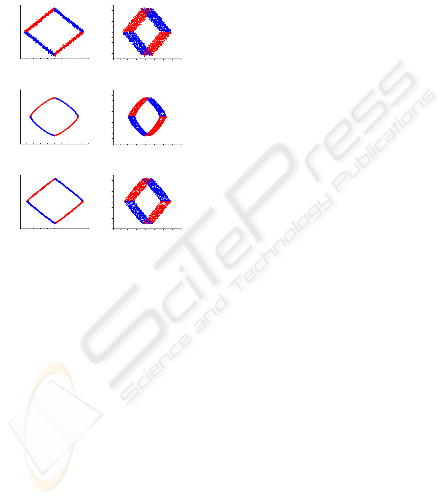
Figure 2: (a-b) Original data, seen from two different views.
(c-d) Results model A, seen from two different views. (e-f)
Results model B, seen from two different views.
3 IMAGE REGISTRATION
For our experiments a Swissranger SR3100 camera
has been used. This new type of sensor has the abil-
ity of simultaneously measuring depth and intensity
for every pixel in the image. The camera is provided
with its own illumination system, composed by a set
of modulated infra-red LEDs. The sensor has a low
pixel resolution of 176 × 144 but a high frame rate
average of 25 fps. This high frame rate makes the
Swissranger camera a suitable sensor for real time ap-
plications.
Depth images of the object are taken for differ-
ent views of the scene. Coarse global registration is
achieved via coarse pose estimation using multiple
correspondences of invariant geometric features ex-
tracted from the 3D point clouds [Chua and Jarvis,
1997]. After the coarse pose registration, an itera-
tive closest point algorithm (ICP) is applied in order
to achieve a fine pose registration [Besl and McKay,
1992].
3.1 TOF Errors and Integration Time
The 3D-Range images captured with TOF sensors
contain different systematic errors that falsify depth
measurements [Oprisescu et al., 2007]. System-
atic errors due to environmental electromagnetic sig-
nals such as sunlight and auto-lighting reflections
have been minimised by restricting the environmen-
tal scene to a suitable non-reflecting uniform textured
one. After recalibration by the manufacturer and fo-
cus distance tuning, short range image extraction has
proved to be appropriate. As a consequence, the in-
trinsic errors due to oversaturation have been consid-
ered as negligible.
One of the TOF sensor parameters that allows to
obtain close range pictures is Integration Time. This
parameter has to be very low in order to assure good
readings from the camera at a range of 30 cm. How-
ever, it adds depth variance into the pixels of the im-
age. In order to deal with this problem the average
of 15 3D-Range images is computed. In order to
enhance the quality of the images, depth discontinu-
ities due to jump edge surfaces are filtered using the
method proposed by [Fuchs and May, 2008].
In the constrained environment of our set-up, the
object is segmented from the background using a
depth threshold.
3.2 Invariant Geometric Feature
Extraction and Rigid Registration
Different invariant geometric feature extraction and
rigid registration methods have been studied and used
in the literature [Seeger and Laboureux, 2000]. We
use a method proposed by Chua and Jarvis (1997).
This method defines rotation and translation invariant
features called “Point Signatures” for every point of a
free-form surface with the benefit that it does not need
partial derivative computations. This approach has
been chosen due to its simplicity and fast behaviour.
4 RESULTS
For parameter choices γ = 0.5, k
n
= 30, k = 1, c =
20/k
n
, and n
i
= 1000, we compute the results of
model A and model B for a synthetic example. Model
B is then applied to the Swissranger sensor data. The
data was scaled by a factor 0.04 before application
of the model, and returned to its original scale after-
wards.
Each aquired data point is assigned a mass point
in the model. We find all k
n
nearest neighbors defin-
ing the neighborhood N(p) of each mass p. The sur-
VISAPP 2009 - International Conference on Computer Vision Theory and Applications
370
face normals are computed by finding k
s
= 12 nearest
neighbors. The neighbors are not altered during the
simulation of the dynamical system.
−20 −15 −10 −5 0 5 10 15 20
−20
−15
−10
−5
0
5
(a) Raw data
−20 −15 −10 −5 0 5 10 15 20
−20
−15
−10
−5
0
5
(b) Coarse registration
−20 −15 −10 −5 0 5 10 15 20
−20
−15
−10
−5
0
5
(c) Fine registration
−20 −15 −10 −5 0 5 10 15 20
−20
−15
−10
−5
0
5
(d) Result model B
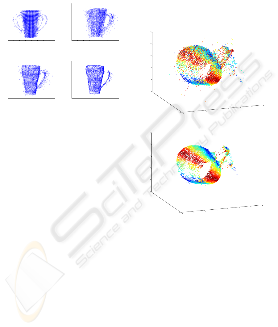
Figure 3: Modeling process of Swissranger data taken from
a mug. (a) Raw data with superimposed unmerged views.
(b) Coarse registration. (c) Fine registration. (d) Final result
using model B.
As a synthetic test example, we choose an object
in the shape of an open box, which is then acquired
from two different view points, separated by an angle
π, via an orthographic projection. We further assume
that the data acquisition process is noisy. In the data
space, the object is represented by a noisy point cloud.
Two different views of this point cloud are shown in
Fig. 2 (a-b). For illustration purposes, we mark all
data points with a surface normal closer to a vector
pointing in the upper left corner as red, and all other
data point as blue. We simulate the dynamical system
of model A for this synthetic example. Two views of
the model data, corresponding to the views shown for
the raw data, are depicted in Fig. 2(c-d). The model
data is much smoother than the original data. How-
ever, since the interaction forces do not take into ac-
count the topology of the object, oversmoothing is
observed at edge discontinuities. Further, the object
model is smaller than the original object. In Fig. 2(e-
f), the result of model B are depicted. Unlike in model
A, the modeled object has the same size as the original
object, and edge discontinuities have been preserved
during the smoothing process.
We apply model B to the depth images of a ce-
ramic mug acquired with the Swissranger sensor. The
different stages of the modeling process, i.e. raw data
acquisition, coarse and fine registration, and results of
the subsequent application of the spring-mass model,
are shown in Fig. 3, a-d, respectively. At the end of
the process, the mug model has a clear shape and most
of the outliers have been removed, except for the han-
dle. In Fig. 4, the color-coded orientations of local
surface patches for the fine registration and the final
result after applying model B are depicted. Surfaces
of mug model B are smoother than the surfaces at the
fine registration stage, thus providing a good basis for
subsequent applications.
−15
−10
−5
0
5
10
15
20
−20
−10
0
10
55
60
65
70
75
80
(a) Fine registration
−15
−10
−5
0
5
10
15
20
−20
−10
0
10
55
60
65
70
75
80
(b) Result model B
Figure 4: Color-coded orientation of local surface patches
for the mug result (a) Fine registration. (b) Final result of
model B.
5 CONCLUSIONS
5.1 Summary
Within the larger context of a robot manipulation task,
we proposed a 3D model for the reconstruction of 3D
objects from Swissranger sensor data. Depth images
are captured with a Swissranger sensor. After tak-
ing depth images from different views, the images
are merged via a coarse registration method [Chua
and Jarvis, 1997]. The shape of the 3D point cloud
is enhanced through application of an iterative clos-
est point algorithm [Besl and McKay, 1992]. The
3D OBJECT RECONSTRUCTION FROM SWISSRANGER SENSOR DATA USING A SPRING-MASS MODEL
371

resulting data is of low resolution and afflicted with
large uncertainties. Modeling the 3D point cloud as
a system of dynamic masses interacting via spring-
like elastic forces reduces these deficiencies. Since
the interaction between masses is dependent on the
orientation of local surfaces fitted to the mass points,
noise and outliers are removed without causing over-
smoothing at edge discontinuities.
5.2 Future Work
Our long-term goal is to model 3D objects during
the execution of a robot task. The proposed model
constitutes a preliminary step before fitting higher-
level surface descriptors which may then be used for
view planning or action selection. The spring-mass
model further provides a framework for modeling de-
formable objects. The outcome of actions can be pre-
dicted by adding an external force to the dynamical
system of the object, e.g. representing a robot grip-
per.
ACKNOWLEDGEMENTS
This work has received support from the BMBF
funded BCCN G¨ottingen, the EU Project PACO-
PLUS under contract FPG-2004-IST-4-027657, and
the Generalitat de Catalunya through the Robotics
group. G. Aleny`a was supported by the CSIC under a
Jae-Doc Fellowship.
REFERENCES
Amenta, N., Bern, M., and Kamvysselis, M. (1998). A
new voronoi-based surface reconstruction algorithm.
In SIGGRAPH ’98, pages 415–421, New York, NY,
USA. ACM.
Besl, P. J. and McKay, N. D. (1992). A method for regis-
tration of 3-d shapes. IEEE Transactions on Pattern
Analysis and Machine Intelligence, 14(2):239–256.
Carr, J., Beatson, R., Cherrie, J., Mitchell, T., Fright, W.,
McCallum, B., and Evans, T. (2001). Reconstruction
and representation of 3d objects with radial basis func-
tions. In Fuime, E., editor, Proceedings of SIGGRAPH
2001, pages 67–76. ACM Press/ACM SIGGRAPH.
Chua, C. S. and Jarvis, R. (1997). Point signatures: a new
representation for 3d object recognition. International
Journal of Computer Vision, 25(1):63–85.
Cuen, S., Andrade, J., and Torras, C. (2008). Action selec-
tion for robotic manipulation of deformable objects.
In Proc. ESF-JSPS Conference on Experimental Cog-
nitive Robotics, Kanagawa.
Curless, B. and Levoy, M. (1996). A volumetric method
for building complex models from range images. In
Proceedings of SIGGRAPH’96.
Fuchs, S. and May, S. (2008). 3d pose estimation and map-
ping with time-of-flight cameras. In Workshop on 3D-
Mapping, IEEE International Conference on Intelli-
gent Robots and Systems (IROS 2008).
Hoppe, H., DeRose, T., Duchamp, T., McDonald, J., and
Stuetzle, W. (1992). Surface reconstruction from un-
organized points. In SIGGRAPH ’92, pages 71–78,
New York, NY, USA. ACM.
Liang, P. and Todhunter, J. S. (1990). Representation
and recognition of surface shapes in range images.
Computer Vision, Graphics and Image Procesing,
52(10):78–109.
Oprisescu, S., Falie, D., Ciuc, M., and Buzuloiu, V. (2007).
Measurements with tof cameras and their necessary
corrections. In Proc. ISSCS, pages 13–14.
Seeger, S. and Laboureux, X. (2000). Feature extraction
and registration: An overview. In Girod, B., Greiner,
G., and Niemann, H., editors, Principles of 3D Im-
age Analysis and Synthesis, pages 153–166, Boston-
Dordrecht-London. Kluwer Academic Publishers.
Szeliski, R., Tonnesen, D., and Terzopoulos, D. (1992).
Modeling surfaces of arbitrary topology with dynamic
particles. CVPR’93, pages 82–87.
Tang, C. and Medioni, G. (2002). Curvature-augmented
tensor voting for shape inference from noisy 3d data.
IEEE Transactions on Pattern Analysis and Machine
Intelligence, 26(6):858–864.
Zhao, H., Osher, S., Merriman, B., and Kang, M.
(2000). Implicit and non-parametric shape reconstruc-
tion from unorganized data using a variational level set
method. In Proceedings of CVIU.
VISAPP 2009 - International Conference on Computer Vision Theory and Applications
372
