A 2D TEXTURE IMAGE RETRIEVAL TECHNIQUE BASED ON

TEXTURE ENERGY FILTERS

Motofumi T. Suzuki, Yoshitomo Yaginuma and Haruo Kodama

National Institute of Multimedia Education, 2-12 Wakaba, Mihama-ku, Chiba-shi 261-0014, Japan

Keywords:

Laws’ ﬁlters, Convolution, 2D Image Database, Image Retrieval, Shape Features.

Abstract:

In this paper, a database of texture images is analyzed by the Laws’ texture energy measure technique. The

Laws’ technique has been used in a number of ﬁelds, such as computer vision and pattern recognition. Al-

though most applications use Laws’ convolution ﬁlters with sizes of 3 × 3 and 5 × 5 for extracting image

features, our experimental system uses extended resolutions of ﬁlters with sizes of 7× 7 and 9 × 9. The use

of multiple resolutions of ﬁlters makes it possible to extract various image features from 2D texture images

of a database. In our study, the extracted image features were selected based on statistical analysis, and the

analysis results were used for determining which resolutions of features were dominant to classify texture

images. A texture energy computation technique was implemented for an experimental texture image retrieval

system. Our preliminary experiments showed that the system can classify certain texture images based on

texture features, and also it can retrieve texture images reﬂecting texture pattern similarities.

1 INTRODUCTION

In the 1990s, intensive research was conducted

on content-based image retrieval methods. Unlike

traditional keyword-based image retrieval methods,

content-based image retrieval methods have used im-

age features as indices for image databases. The im-

age features describe characteristics of the images

which include colors, shapes and textures. Since im-

age feature indices can be extracted automatically by

using software programs, this process is more ef-

ﬁcient and faster compared to that of keyword in-

dices which are assigned by human hands. Various

image feature extraction techniques have been pro-

posed based on computer algorithms, such as co-

occurrence matrices (Haralick et al., 1973), Markov

random ﬁeld modeling (Cross and Jain, 1983), Gabor

ﬁltering (Manjunath and Ma, 1996), Wavelet (Chang

and Kuo, 1993), and HLAC (Kato, 1992). Also, vari-

ous statistical learning techniques have been proposed

to improve retrieval rates by learning from the sam-

ple image data (Kato, 1992). Such techniques include

use of self-organizing maps (SOM), neural networks

(NN) and support vector machines (SVM). Details of

image features and a related retrieval technique sur-

vey can be found in several papers (Veltkamp and

Tanase, 2000) (Datta et al., 2008).

In our experiments, the famous Laws’ texture en-

ergy measure technique is applied to a 2D texture

image database. Although a typical application uses

Laws’ ﬁlters of 3× 3 and 5× 5, the sizes of the ﬁlters

were extended to 7× 7 and 9 × 9 in our experiments.

These multiple resolutions of the ﬁlters were used for

extracting image features from images of a texture

database. The extracted features were analyzed by

linear discriminant analysis to determine which res-

olutions of features were best suited for classifying

the texture database. Also, principal component anal-

ysis (PCA), and the k-nearest neighbor (KNN) algo-

rithm was used for the similarity retrieval of a texture

database.

2 TEXTURE ENERGY FILTERS

In this section, (1) Laws’ texture energy measures, (2)

convolution and (3) rotation invariant features are dis-

cussed.

2.1 Laws’ Texture Energy Measures

The texture analysis technique based on the texture

energy measure which was developed by K. I. Laws

145

T. Suzuki M., Yaginuma Y. and Kodama H. (2009).

A 2D TEXTURE IMAGE RETRIEVAL TECHNIQUE BASED ON TEXTURE ENERGY FILTERS.

In Proceedings of the First International Conference on Computer Imaging Theory and Applications, pages 145-151

DOI: 10.5220/0001820701450151

 SciTePress

(Laws, 1979) (Laws, 1980) has been used for many

applications of image analysis for classiﬁcation and

segmentation. The texture energy measurements for

2D images are computed by applying convolution ﬁl-

ters. In the technique, three basic ﬁlters were used as

follows:

L3 = (1 2 1)

E3 = (-1 0 1)

S3 = (-1 2 -1)

The initial letters of these ﬁlters indicate Local av-

erage (or Level), Edge detection, and Spot detection.

The numbers followed by the initial letters indicate

lengths of the ﬁlters. In this case, the length of the

ﬁlters is three. Often, extended lengths of ﬁlters are

used for 2D image analysis. The extension of the ﬁl-

ters can be done by convolving the pairs of these ﬁl-

ters together. For example, ﬁlters with a length of ﬁve

can be obtained by convolving pairs of ﬁlters with a

length of three. In this convolution process, nine ﬁl-

ters (3 × 3) can be formed, and ﬁve of them are dis-

tinct. The following is a set of one dimensional con-

volution ﬁlters of a length of ﬁve:

L5 = (1 4 6 4 1)

E5 = (-1 -2 0 2 1)

S5 = (-1 0 2 0 -1)

W5 = (-1 2 0 -2 1)

R5 = (1 -4 6 -4 1)

The initial letters of these ﬁlters stand for Local

average (or Level), Edge, Spot, Wave, and Ripple.

All ﬁlters are zero-sum ﬁlters except for the L5 ﬁl-

ter. Many applications use Laws’ ﬁlter with a size of

3 and 5 for extracting texture energyvalues. In our ex-

periments, we have extended the ﬁlter sizes to 7 and

9. The ﬁlters of 7 can be obtained by convolving ﬁl-

ters of a length of ﬁve and ﬁlters of a length of three

as follows:

Xa7 = ( 1, 6, 15, 20, 15, 6, 1 )

Xb7 = ( 1, 4, 5, 0, -5, -4, -1 )

Xc7 = ( -1, -2, 1, 4, 1, -2, -1 )

Xd7 = ( 1, 0, -3, 0, 3, 0, -1 )

Xe7 = ( 1, -2, -1, 4, -1, -2, 1 )

Xf7 = ( 1, -4, 5, 0, -5, 4, -1 )

Xg7 = ( -1, 6, -15, 20, -15, 6, -1 )

By using a similar approach, one dimensional ker-

nels of a length of nine are obtained as follows:

All the kernels are zero-sum kernels except for

Xa7 and Ya9. Simple sequential labels X and Y were

assigned for the ﬁlters 7 and 9 for convenience, al-

though more meaningful labels such as L, E, S, W

Ya9 = ( 1, 8, 28, 56, 70, 56, 28, 8, 1 )

Yb9 = ( 1, 6, 14, 14, 0, -14, -14, -6, -1 )

Yc9 = ( -1, -4, -4, 4, 10, 4, -4, -4, -1 )

Yd9 = ( 1, 0, -4, 0, 6, 0, -4, 0, 1 )

Ye9 = ( 1, 2, -2, -6, 0, 6, 2, -2, -1 )

Yf9 = ( -1, 2, 2, -6, 0, 6, -2, -2, 1 )

Yg9 = ( -1, 4, -4, -4, 10, -4, -4, 4, -1 )

Yh9 = ( 1, -8, 28, -56, 70, -56, 28, -8, 1 )

Yi9 = ( 1, -6, 14, -14, 0, 14, -14, 6, -1 )

and R can be used. (Obviously, Xa7 can be labeled

L7, and Ya9 can be labeled L9.)

These one dimensional ﬁlters are used to gener-

ate two dimensional ﬁlters by combining these one

dimensional ﬁlters. The set of two dimensional ﬁlters

with lengths of three (3× 3) are as follows:

L3L3, L3E3, L3S3

E3L3, E3E3, E3S3

S3L3, S3E3, S3S3

In a similar manner, two dimensional ﬁlters with

the lengths of 5 × 5, 7 × 7 and 9 × 9 can be ob-

tained. Furthermore, three dimensional ﬁlters such as

3 × 3 × 3 can be generated by combining basic one

dimensional ﬁlters (Suzuki and Yaginuma, 2007).

2.2 Convolution

Once the two dimensional ﬁlters are obtained, these

ﬁlters are used to convolve the 2D texture image. The

convolution of image I and ﬁlter F with a size of 2t +

1 by 2t + 1 is expressed by the following equation:

R(i, j) = F(i, j)∗I(i, j) =

∑

k=−t

∑

l=−t

F(k,l)I(i+k, j+l)

(1)

where ’∗’ denotes two dimensional convolution com-

putation. For the next step, the windowing process

is applied to convolved images. In this process, tex-

ture energy values are computed. Every pixel in the

convolved images is replaced with a texture energy

measure value at the pixel. In the Laws’ paper, a

15 × 15 square around each pixel is added together

with the values of the neighborhood pixels. In this

computation, Laws introduced ”squared magnitudes”

and ”absolute magnitudes” to compute texture energy

(Laws, 1979) (Laws, 1980). For considering compu-

tation efﬁciency, ”absolute magnitude” is used in gen-

eral. This computation process can be expressed by

the following equation:

E(l,m) =

l+t

∑

i=l−t

m+t

∑

j=m−t

|K(i, j)| (2)

IMAGAPP 2009 - International Conference on Imaging Theory and Applications

146

where K is the local features, and it is smoothed at

position (l,m) by using a (2t + 1) × (2t+ 1) window.

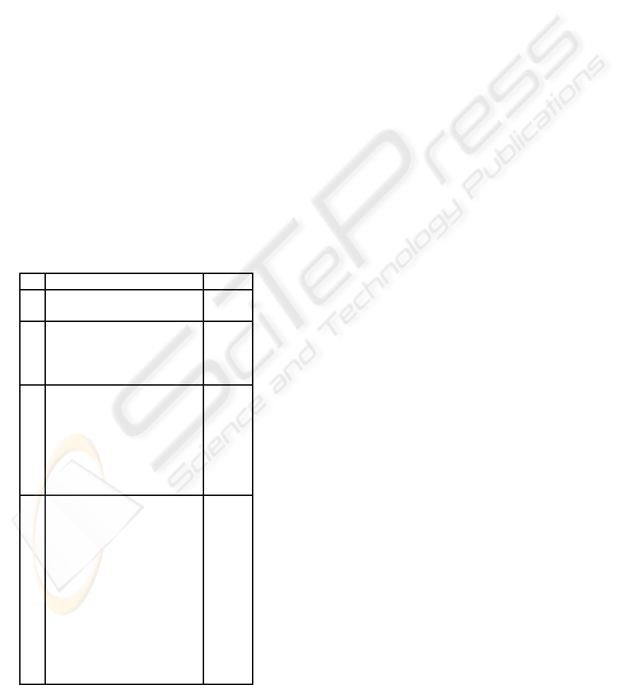
2.3 Rotation Invariant Features

Some ﬁlters are identical if they are rotated 90 de-

grees. The features which are computed from the ﬁl-

ters can be combined as similar features, and these

features are treated as rotation invariant features in

the order of 90 degrees. For example, feature E5L5

can be combined with L5E5, and newly created fea-

tures are denoted as E5L5

where R means the ”ro-

tation invariant” feature. On the other hand, some

features such as E5E5, S5S5, W5W5 and R5R5 can

not be combined. Since the rotation invariant fea-

tures were combined with two features, the feature

values were scaled by 2. Therefore, the rotation in-

variant features are divided by 2 for the purpose of

normalization. Figure 1 shows rotation invariant fea-

tures for ﬁlter lengths of 3× 3, 5× 5, 7× 7 and 9× 9.

(In this paper, rotation invariant features are denoted

as 3 × 3

, 5 × 5

, 7 × 7

and 9 × 9

, respectively.)

Also the number of corresponding rotation invariant

features is shown in Figure 1. The number of rota-

tion invariant features F

can be computed by equa-

tion F

= n

− ((n

− n)/2) where n is ﬁlter size.

R. Rotation Invariant Features Num.

L3L3,L3E3

,L3S3

,E3E3 9 → 6

E3S3

,S3S3

L5L5,L5E5

,L5S5

,L5R5

25 → 18

L5W5

,E5E5,E5S5

,E5R5

E5W5

,S5S5,S5R5

,S5W5

R5R5,R5W5

,W5W5

XaXa7,XaXb7

,XaXc7

,XaXd7

49 → 28

XaXe7

,XaX f7

,XaXg7

,XbXb7,

XbXc7

,XbXd7

,XbXe7

,XbX f7

XbXg7

,XcXc7, XcXd7

,XcXe7

XcX f7

,XcXg7

,XdXd7,XdXe7

XdX f7

,XdXg7

,XeXe7, XeX f 7

XeXg7

,X f X f7,X fXg7

,XgXg7

YaYa9,YaY b9

,YaY c9

,YaYd9

81 → 45

YaYe9

,YaY f9

,YaY g9

,YaY h9

YaYi9

,YbYb9,YbYc9

,YbYd9

YbYe9

,YbY f9

,YbYg9

,YbYh9

YbYi9

,YcYc9,YcYd9

,YcYe9

YcY f 9

,YcYg9

,YcYh9

,YcYi9

YdYd9,YdYe9

,YdY f9

,YdYg9

YdYh9

,YdYi9

,YeYe9,YeY f9

YeYg9

,YeYh9

,YeYi9

,Y fY f9

Y fYg9

,Y fY h9

,Y fYi9

,YgYg9

YgYh9

,YgYi9

,YhYh9,YhYi9

YiYi9

Figure 1: Rotation invariant features (3×3

, 5×5

, 7×7

and 9× 9

3 EXPERIMENTS AND RESULTS

This section describes (1) experimental textures, (2)

comparison of ﬁlters for various lengths, (3) similar-

ity retrievals of a texture database

3.1 Experimental Textures

In our experiment, a portion of the OUTEX (Ojala

et al., 2002) texture database was used. It contains

6380 textures (Outex-TR-00000 data set). It consists

of 319 classes of textures with 20 textures in each

class. The database contains both macro-textures and

micro-textures. Texture sizes are 128 × 128 in RAS

image data format. In our experiments, these data are

converted to sizes of 128 × 128 images in PGM for-

mat with 65536 grey scale colors.

3.2 Comparison of Filters for Various

Lengths

Various lengths of Laws’ ﬁlters were examined to de-

termine whether the ﬁlters can classify the textures.

For the experiments, ﬁve classes of textures were se-

lected from a portion of the OUTEX database. The

examples of the textures are shown in Figure 2. Each

class contains 20 textures, thus there were a total of

100 textures. Figure 3 shows examples of convolved

texture images (seeds textures) using Laws’ ﬁlters

(3 × 3, 5 × 5 and 7 × 7). As the ﬁlter sizes are in-

creased, the resolutions of the convolved images be-

come coarser. Texture images analyzed by large size

ﬁlters such as 7 × 7 contain very similar convolved

texture images. Some features associated with these

similar convolved images are considered redundant,

and these convolved images can be eliminated for ef-

ﬁcient computation. The elimination of the redundant

features avoids a bias from the features due to dimen-

sionality.

Once the entire texture data were analyzed by

Laws’ ﬁlters, the texture energycould be computed by

the technique mentioned in the previous section (Sec-

tion 2). For the texture energy computation, 15 × 15

smoothing windows were used for the experiments.

These texture energy values and texture class iden-

tiﬁcation numbers were used as input of a discrim-

inant analysis (LDA). In this experiment, Laws’ ﬁl-

ters of sizes 3 × 3, 5 × 5, 7 × 7 and 9 × 9 were ex-

amined. For each ﬁlter size, rotation invariant (men-

tioned in section 2.3) features (3× 3

, 5 × 5

, 7 × 7

and 9×9

) were also computed. Ten textures for each

class were used for the learning data sets (10 textures

× 5 classes).

A 2D TEXTURE IMAGE RETRIEVAL TECHNIQUE BASED ON TEXTURE ENERGY FILTERS

147

Seeds

Paper

Pasta

Figure 2: Example of textures.

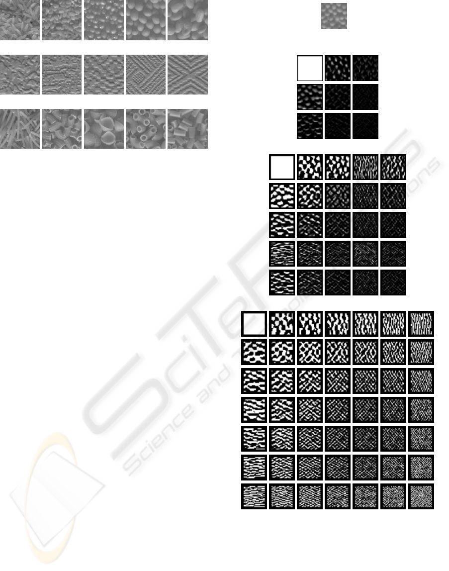
Figure 4 shows texture data of discriminant co-

ordinates for features based on the Laws 7 × 7 ﬁlter.

Four discriminant functions are labeled LD1, LD2,

LD3 and LD4 in the ﬁgure. The labels a, b, c, d and

e in the ﬁgure indicate each class of textures. When

each function has good discriminating power, there is

no overlap observed between texture classes.

Figure 5 shows proportions of eigenvalues for the

discriminant functions. The eigenvalues reﬂect the

amount of variance explained in the grouping vari-

ables by the predictors. In the ﬁgure, the proportion

of the eigenvalues estimates the relative importance

of the discriminant functions. In the case of the ﬁg-

ure, discriminant functions LD1, LD2, and LD3 have

more discriminating power compared to that of LD4.

The larger the coefﬁcient values of a predictor in

the discriminant function, the more important its role

in the discriminant function. Therefore, these predic-

tors (image features) associated with the larger coef-

ﬁcients are inﬂuential predictors (image features) for

classifying textures. In this example, features XeXe7,

X fXd7 and X fX f7 had relatively large coefﬁcients

for the LD1 function, and they are considered as im-

portant image features for classifying our experimen-

tal texture dataset. Important image features vary de-

pending on the patterns which are contained in the

texture dataset.

Figure 6 shows a set of test texture data (tex-

tures of seeds) classiﬁed by the discriminant func-

tions trained by the training data set. In the ﬁgures,

rows represent predicted texture types, and columns

represent actual texture types. For the 5 × 5 ﬁlter

case, there are 4 textures misclassiﬁed. Two percent

(1/50) of ’a’ textures are misclassiﬁed as ’f’ textures,

2% (1/50) of ’b’ textures are misclassiﬁed as ’e’, 2%

(1/50) of ’d’ textures are misclassiﬁed as ’c’, and 2%

(1/50) of ’e’ textures are misclassiﬁed as ’d’, There-

fore, 92% (46 out of 50) of test textures are classiﬁed

Source texture image

3× 3

5× 5

7× 7

Figure 3: Examples of convolved texture images using

Laws’ ﬁlters (3× 3, 5× 5 and 7× 7).

correctly for the 5 × 5 ﬁlter. The classiﬁcation rates

for each ﬁlter can be computed in a similar manner,

and the rates are shown in Figure 7. As shown in Fig-

ure 7, ﬁlters 5×5, 7×7, 7×7

, 9×9 and 9× 9

show

fair classiﬁcation rates.

IMAGAPP 2009 - International Conference on Imaging Theory and Applications

148

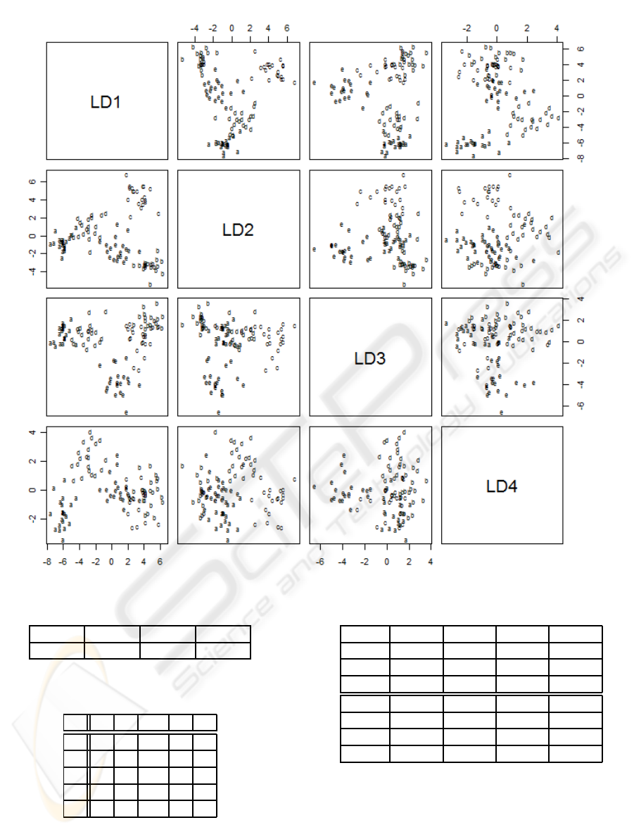
Figure 4: Texture data of discriminant coordinates for features of the 7× 7 ﬁlters.

LD1 LD2 LD3 LD4

0.5928 0.1757 0.1460 0.0855

Figure 5: Proportions of eigenvalues for discriminant func-

tions (7× 7 ﬁlters).

a b c d e

a 9 0 0 1 0

b 0 9 0 0 1

c 0 0 10 0 0

d 0 0 1 9 0

e 0 0 0 1 9

Figure 6: Classiﬁcation rate tables for ﬁlters 5 × 5 (Seeds

textures).

3.3 Similarity Retrievals of a Texture

Database

Experiments on similarity retrievals of a texture

database have been conducted. The Laws’ ﬁlters

3×3 5 ×5 7×7 9×9

Seeds 42.0% 92.0% 100.% 96.0%

Paper 56.0% 90.0% 100.% 96.0%

Pasta 56.0% 86.0% 100.% 94.0%

3× 3

5× 5

7× 7

9× 9

Seeds 42.0% 62.0% 78.0% 100.%

Paper 38.0% 56.0% 90.0% 100.%

Pasta 30.0% 64.0% 94.0% 100.%

Figure 7: Classiﬁcation rates for ﬁlters 3 × 3, 5× 5, 7× 7,

9× 9, 3× 3

, 5× 5

, 7× 7

, 9× 9

(3× 3, 5 × 5, 7 × 7 and 9 × 9) have been applied to

the database to extract texture image features. Also,

rotation invariant features (3× 3

, 5 × 5

, 7 × 7

and

9 × 9

) have been computed. The database contains

6380 textures (128× 128; 20 images × 319 classes),

A 2D TEXTURE IMAGE RETRIEVAL TECHNIQUE BASED ON TEXTURE ENERGY FILTERS

149

and the image feature extraction computation took

about six hours using a standard computer (Intel (R)

Core 2 Duo E8600 processor). The extracted fea-

tures were analyzed by principal component analysis

(PCA). The PCA transforms a number of correlated

features into a smaller number of uncorrelated fea-

tures called principal components. The PCA reduces

the dimensionality of the data set without a signiﬁcant

loss of information. Since our image feature data sets

contain redundant features for higher resolution ﬁlters

such as 7 × 7 and 9 × 9, the redundant features can

be eliminated by applying the PCA. For our texture

retrieval system, the dimensions of the feature space

were reduced. All the dimensions of the feature space

were reduced so that the features kept over 90% of

their information.

The k-nearest neighbor algorithm (KNN) was

used for retrieving texture from the database. A tex-

ture was classiﬁed by a majority vote of its neighbors,

with the texture being assigned to the class most com-

mon amongst its k nearest neighbors.

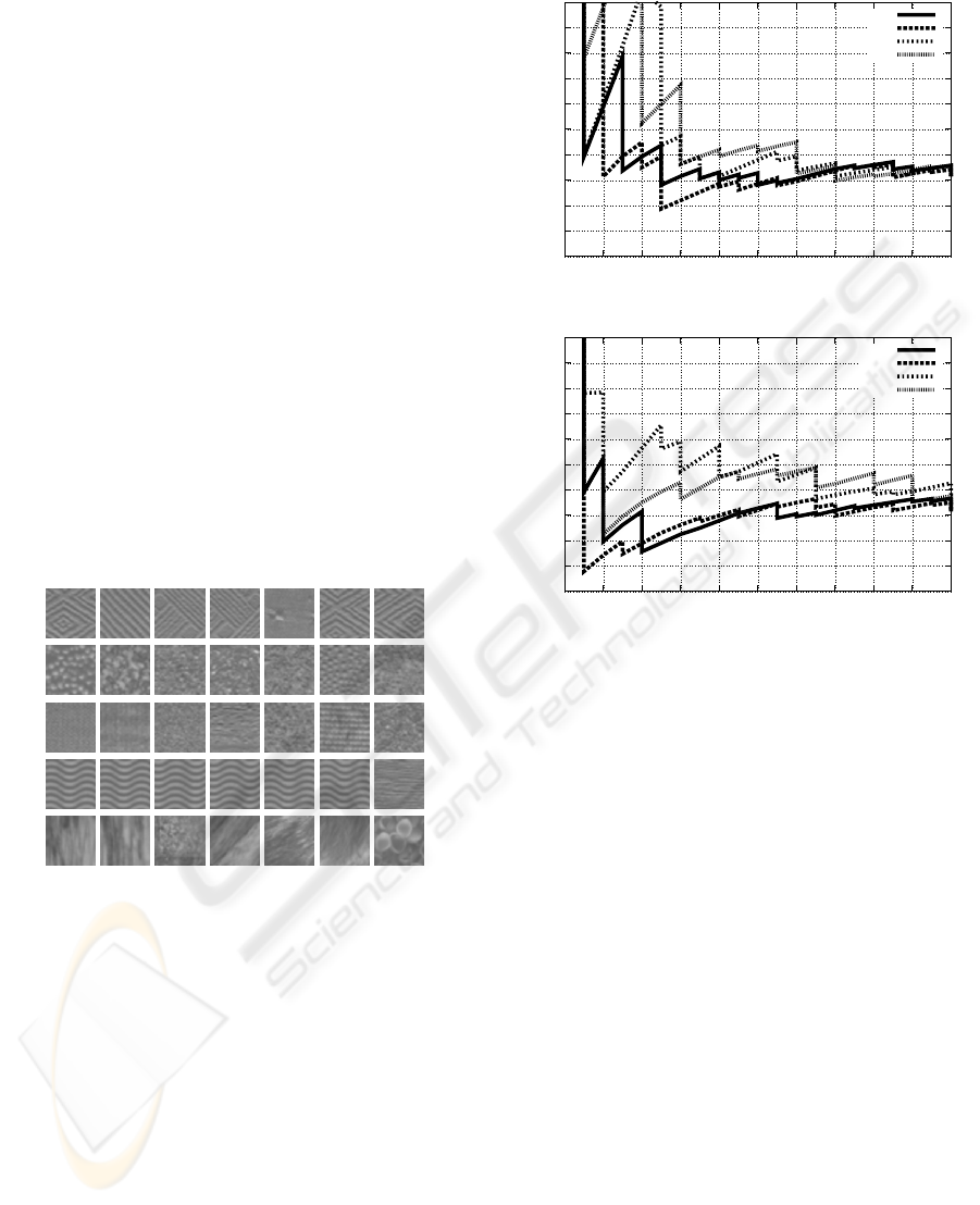
Figure 8 shows examples of the similarity retrieval

of textures. In each ﬁgure, the six most similar tex-

tures determined by the system are shown.

Figure 8: Similarity retrieval of textures (In each ﬁgure, the

left image shows the query key).

Figure 9 shows a Recall-Precision graph for the

retrieval test. In the experiment, 20 random query

keys were selected, and corresponding recall rates and

precision rates were computed.

In the ﬁgure, ﬁlters 7× 7, 7× 7

, 9× 9 and 9× 9

show good retrieval results compared to other ﬁlters

when our experimental database is examined.

0.1

0.2

0.3

0.4

0.5

0.6

0.7

0.8

0.9

0 10 20 30 40 50 60 70 80 90 100

Precision (%)

Recall (%)

Recall-Precision

3x3

5x5

7x7

9x9

0.1

0.2

0.3

0.4

0.5

0.6

0.7

0.8

0.9

0 10 20 30 40 50 60 70 80 90 100

Precision (%)

Recall (%)

Recall-Precision

3x3R

5x5R

7x7R

9x9R

Figure 9: Recall-Precision graph for the retrieval test.

4 CONCLUSIONS AND FUTURE

WORK

Two dimensional image textures were analyzed by the

Laws’ texture energy measure approach. Various res-

olutions of Laws’ ﬁlters (3× 3, 5× 5, 7× 7 and 9× 9)

were used for extracting image features. Also, ro-

tation invariant features (3 × 3

, 5 × 5

, 7 × 7

and

9×9

) were computed. A database of a texture image

was analyzed using a simulation software program. In

the experiments, classiﬁcation rates of the Laws’ ﬁl-

ters were evaluated, and textures were classiﬁed fairly

well when the ﬁlters were used in conjunction with

the discriminant analysis. A principal component

analysis (PCA) and a k-nearest neighbor (KNN) al-

gorithm were used for the similarity retrieval. Use of

these statistical techniques reduced unnecessary im-

age features, and made possible the retrieval of pat-

tern similar textures from the database.

For future experiments, additional 2D textures

which contain various patterns will be examined.

Other statistical approaches such as a quadratic dis-

criminant analysis will be applied in conjunction with

the Laws’ ﬁlters for improving classiﬁcation rates.

IMAGAPP 2009 - International Conference on Imaging Theory and Applications

150

Also, other ﬁltering techniques (Randen and Husoy,

1999) will be examined for content-based image re-

trieval.

ACKNOWLEDGEMENTS

This research was partially supported by grants

from the Telecommunications Advancement Foun-

dation, Japan (TAF-2007) and the KAKENHI (YR-

19700108).

REFERENCES

Chang, T. and Kuo, C. J. (1993). Texture analysis and clas-

siﬁcation with tree-structured wavelet transform. In

IEEE Trans. Image Process. 2 (4), pp.429–441.

Cross, G. and Jain, A. (1983). Markov random ﬁeld texture

models. In IEEE Trans. Pattern Anal. Mach. Intell. 5

(1), pp.25–39.

Datta, R., Joshi, D., Li, J., and Wang, J. Z. (2008). Image

retrieval: Ideas, inﬂuences, and trends of the new age.

In ACM Computing Surveys, vol. 40, no. 2.

Haralick, R. M., Shanmugam, K., and Dinstein, I.

(1973). Textural features for image classiﬁcation. In

IEEE Trans. Sysmtems Man Cybernetics,Vol.3, No.6,

pp.610–621. IEEE.

Kato, T. (1992). Database architecture for content-based

image retrieval. In Proc. SPIE Image Storage Re-

trieval System, 1662, pp.112–123.

Laws, K. I. (1979). Texture energy measures. In DARPA

Image UnderstandingWorkshop, pp.47–51. DARPA.

Laws, K. I. (1980). Rapid texture identiﬁcation. In Im-

age Processing for Missile Guidance, SPIE Vol. 238,

pp.376–380.

Manjunath, B. and Ma, W. (1996). Texture features for

browsing and retrieval of image data. In IEEE Trans.

Pattern Anal. Mach. Intell. 18 (8), pp.837–842.

Ojala, T., Maenpaa, T., Pietikainen, M., Viertola, J., Kyllo-

nen, J., and Huovinen, S. (2002). Outex - new frame-

work for empirical evaluation of texture analysis algo-

rithms. Proc. 16th International Conference on Pattern

Recognition, Quebec, Canada, pp.701–706.

Randen, T. and Husoy, J. (1999). Filtering for texture clas-

siﬁcation: a comparative study. In Pattern Analysis

and Machine Intelligence, IEEE Transactions on Vol.

21, Issue 4, pp.291-310. IEEE.

Suzuki, M. T. and Yaginuma, Y. (2007). A solid texture

analysis based on three dimensional convolution ker-

nels. In Electronic Imaging 2007, Videometrics IX,

(EI-2007), Proc. of SPIE and IST Electronic Imaging,

SPIE Vol. 6491, 64910W pp.1–8.

Veltkamp, R. C. and Tanase, M. (2000). Content-based im-

age retrieval systems: A survey. In Technical Report

UU-CS-2000-34. Institute of Information and Com-

puting Science, University Utrecht.

A 2D TEXTURE IMAGE RETRIEVAL TECHNIQUE BASED ON TEXTURE ENERGY FILTERS

151