ROBOT SELF-LOCALIZATION
Using Omni-directional Histogram Correlation
William F. Wood, Arthur T. Bradley, Samuel A. Miller and Nathanael A. Miller
NASA Langley Research Center, 5 N. Dryden St., Hampton, VA 23681 U.S.A.
Keywords: Self-localization, Omni-directional, Histograms.
Abstract: In this paper, we describe a robot self-localization algorithm that uses statistical measures to determine color
space histograms correlations. The approach has been shown to work well in environments where spatial
nodes have unique visual characteristics, including rooms, hallways, and outdoor locations. A full color
omni-directional camera was used to capture images for this localization work. Images were processed
using user-created algorithms in National Instrument’s LabView software development environment.
1 INTRODUCTION
The ability for a robot to locate itself in a local or
global frame gives a unique positional awareness
that leads to better navigational choices, optimized
path planning, and topological mapping. One type of
robot localization is to rely on external sources (e.g.
GPS, internet access, human input, etc.) to inform
the robot of its relative and perhaps absolute
position. For remote missions however, with areas
that are inaccessible, previously unexplored, have
lengthy control delays, or have no support structure
available, the robot must perform self-localization.
Our goal in investigating robot self-localization was
to mimic a human’s ability to determine his/her
location – generally done using a combination of
sensory inputs and historical references. Topological
localization of this type requires that a robot learn its
environment, creating its own database of unique
locations as well as a nodal map showing how the
locations are interconnected.
Our work builds on previous research in which
an omni-directional camera was used for histogram
correlation (Ulrich, 2000) (Abe, 1999). Our research
selects the best of three statistical measures with an
averaging process to better perform scene
recognition. The averaged approach leads to
different scoring and voting systems, and requires
fewer images per node to achieve acceptable results.
The method of histogram correlation is first
introduced. Existing as well as new algorithms are
then discussed using both equations and a flow
chart. And finally the results of correlating for
several locations are examined.
2 HISTOGRAMS
There are many possible methods for self-
localization, including approaches based on colors,
sound, infrared images, range signatures, and object
recognition. We used color histogram matching,
because it was believed to closely emulate a
human’s ability to perform area recognition by broad
color differentiation. The approach uses four
primary color spaces, each with three 8-bit color
bands: Red, Green and Blue (RGB); Hue, Saturation
and Luminosity (HSL); Hue, Saturation and Value
(HSV); and Hue, Saturation and Intensity (HSI), as
well as normalized versions of those spaces.
Normalized color spaces are created by normalizing
the individual color bands with the total color value.
For example, normalized RGB would be calculated
using (1).





(1)
Where NX is the normalized value and X can be R,
G, or B.
Processing full color images require a great deal
of processing capability and memory. Therefore all
images were converted into color histograms before
correlation. Histograms are typically two-
dimensional representations of the distribution of

colors in an image. One axis of the histogram
corresponds to the color bins (e.g. shades of red –
dark to light), and the other axis corresponds to the
number of pixels in the image that fall in this color
bin. It serves as a statistical description of the
occurrence of different color regions and is often
used by photographers to prevent over/under
exposure.
Consider an image captured using the RGB color
space. Three separate histograms are created, one for
each color band (R, G, B). The histogram for the R
band is shown in Figure 1. For this particular
histogram, we can see that the single red line
represents the red 8-bit color band. The horizontal
axis value of 0 translates to the zero brightness bin
(usually indicating a black color). Likewise, the
horizontal value of 255 indicates the maximum
brightness bin. In this case, the red peak occurs at a
bin value of ~97. Also note that a second peak
occurs at the value of 255 indicating that there is
some white content to the image.
Figure 1: Sample histogram of R band.
The obvious advantage of converting images to a
descriptive histogram is the significant file size
reduction. A full color 16-bit resolution 640 x 480
image requires about 4.92 Mb of memory (assuming
uncompressed data). Whereas the same image
described as three histograms require only 6.1 kb (8-
bit count x 255 bins x 3 bands). Reduced file sizes
make both data storage and image correlation much
less intensive. Furthermore, the histogram size is
independent of the image size, making algorithms
easily transportable between systems.
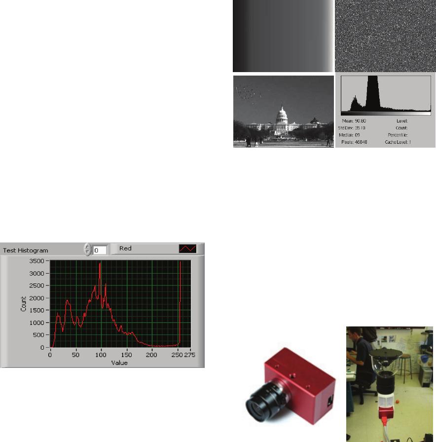
The disadvantage of histograms is that they are
representations of color only, and have no
information about object shape or texture. For that
reason, completely different images can theoretically
have identical histograms as seen in Figure 2.
In practice however, we have found that the
histogram of a complex space (e.g. a cluttered room
or parking lot) is quite unique and can be used for
self localization.
Figure 2: Three images share same histogram (bottom
right).
3 IMAGE CAPTURE
For this investigation, we used a camera system with
an omni-directional field of view (FOV). Omni-
directional images are insensitive to rotation and
work well when combined with histograms, which
are insensitive to translation and inclination. It also
allows for a single image to capture an entire
location. As shown in Figure 3, the omni-directional
FOV was achieved using a CCD VGA camera and a
parabolic mirror.
Figure 3: Videre Designs CCD camera and SOIOS omni-
directional mirror.
One shortcoming of our camera was that it does
not have either auto-brightness or auto-focus
controls. The brightness issue was remedied by
using an auto-brightness control algorithm.
However, we were forced to use a manual single
fixed focal length for the experiment. In a practical
system, auto focus would be a beneficial for reliable
localization.
LabVIEW 8.5 by National Instruments was used
for analysis and to communicate with the camera via
an IEEE 1394 interface. LabVIEW provides an
object-oriented programming environment to easily

convert images to histograms and perform statistical
correlation.
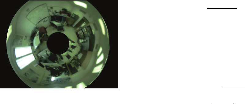
Images taken by the omni-directional camera
appear as “donut-shaped,” with a dead space in the
center corresponding to the parabolic reflection of
our lens and mounting assembly. Figure 4 shows a
sample image from our camera system.
Figure 4: Sample omni-directional image.
The black rectangular border (caused by the CCD
shape) and the vertex dead space were removed by a
masking algorithm, preventing them from being
used in the image-to-histogram conversions.
4 STATISTICAL
HISTOGRAM-MATCHING
The concept on statistical histogram matching was
reported by a group of researchers at Carnegie
Mellon University (Ulrich, 2000). Their work uses
three statistical measures to correlate histograms: χ2,
Jeffrey divergence (JD), and Kolmogorov-Smirnov
(KS). We used the same statistical measures in our
research. They are briefly discussed below
(Papoulis, 2002).
4.1 χ2 Statistics
The χ2 method is a bin-by-bin histogram distance
difference calculation. H and K are sets of color
histograms from two comparing images. They can
be from any color space: RGB, HSV, HSL or HSI.
However to correlate them, both histogram sets must
describe the same color space. Let elements h
ij
and
k
ij
describe the individual entries of H and K, where
i represents the bin number and ranges from 0 to 255
and j represents the particular color band (e.g. R, G,
or B if RGB space is being used).
By this definition, there are three sets of h
i
and k
i
pairs. For example in RGB case, there are h
iR
, k
iR
,
h
iG
, k
iG
and h
iB
, k
iB
. The distance between the two
histograms is defined by (2) and is a normalized
measure of how well the two histograms correlate
across all three color bands. Perfect correlation
would yield a distance of zero.


,










,
(2)
4.2 Jeffrey Divergence (JD) Statistics
The Jeffrey Divergence method is also a bin-by-bin
histogram distance difference calculation. Using the
same notation as defined with
χ 2, the distance
between two histograms is given by (3).


,



·


2·






,


·


2·






,
(3)
Once again the distance between two identical
images would be zero.
4.3 Kolmogorov-Smirnov (KS)
Statistics
The Kolmogorov-Smirnov method is a third
statistical measure, one that looks for the greatest
difference between bins. The distance is then given
by (4).


,






(4)
5 IMAGE CORRELATION
To perform self-localization, the robotic system
must first capture one or more training images for
each location. This can be done a priori in a
controlled manner, or dynamically as the robot first
maps an unexplored area. The training images
(stored as histograms) are kept in a database and
used to correlate against real-time images (also
converted to histograms), helping the robot to
determine its location.
When performing self-localization, the robot
correlates one or more real-time images (perhaps
taken from different vantage points in a location)
with the training images for every known location

(a.k.a. nodes). In the most favorable case, the robot
would have numerous training images for every
location to help with correlation accuracy.
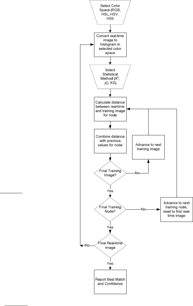
The process of correlating an image is illustrated
as a flow diagram in Figure 5. The test image is first
converted to a histogram of the appropriate color
space. A statistical method is then selected. Next, the
distance between the test image and each training
image of a given node is calculated. The distances
between the test image and all training images for
that node are then averaged. The process is repeated
across all training nodes, with each training node
yielding a distance result. If additional test images
are available, the correlation process is repeated,
with the results averaged with those from the first
test image correlation.
Mathematically, the formulas to perform location
recognition are best presented in operational stages.
The distance between a single test image and a
single training image is calculated by one of the
three statistical distance equations (2), (3), (4).
Additional test-to-training distances are calculated
and combined for every training image in a node.
The combined distance between a test image and all
images in a training node is defined by the
following.



,




,
3

(5)
Where x is the training node number, n is the
number of training images, and 3 averages across the
three color bands. The result is an averaged distance
indicating how well a single test image correlates to
multiple training images from node x. This process
is repeated across all nodes, yielding a set of
distance values between the image and each training
node.
If more than one test image is available, the
process is repeated with the results again averaged.
In this case, the result is a set of total distances
between a group of test images and each of the
training nodes.



,




,


(6)
Figure 5: Correlation process.
Where m is the number of test images and x is
the training node.
For each statistical method, the single formula
representations for the total distance between a set of
test images and a set of training images from a
training node are given in the final section by (8),
(9), and (10).

6 CONFIDENCE
DETERMINATION
Each test image is ultimately identified as a
particular training location based on which one it
best matched. If multiple test images are available,
then a correlation confidence is calculated.

#ofimagesagreeingonlocation
#oftestimages
(7)
For example if there are 10 test images, and 9 of
them agree on the location (based on correlation
results), then the confidence is calculated as 90%.
The selection process can be made more robust by
performing the distance calculations using all three
statistical methods and then selecting the location
based on the method that yields the highest level of
confidence. Likewise, calculations can be made for
more than one color space (RGB, HSL, etc.) and the
best results selected.
7 RESULTS
The test set up was consistent for all images, with
fixed camera height and focus. Also, the nodes
remained generally unchanged without the presence
of numerous people or other dynamic objects. The
omni-directional lens removed the need to consider
camera orientation. Finally, the RoboticVision
program performed auto-brightness to eliminate
significant light variations.
Testing consisted of first capturing 15 training
images for 10 different locations (a.k.a. nodes).
Obviously, the greater the number of nodes, the
more difficult the final correlation. Likewise, the
greater the number of training images, the easier the
correlation. Training nodes consisted of 6 rooms, 1
hallway, and 3 outdoor locations.
The robot then maneuvered to each location of
interest collecting 15 test images before performing
correlation. Fewer training and test images are
certainly possible, but the increased number helped
to make the correlation more robust. Test and train
images were also taken on the same day to help
reduce dynamic changes (e.g. light, objects moved,
etc.) that might have occurred to the locations. We
realize this is an oversimplification, but the goal was
to prove the initial theory before introducing
additional uncertainties.
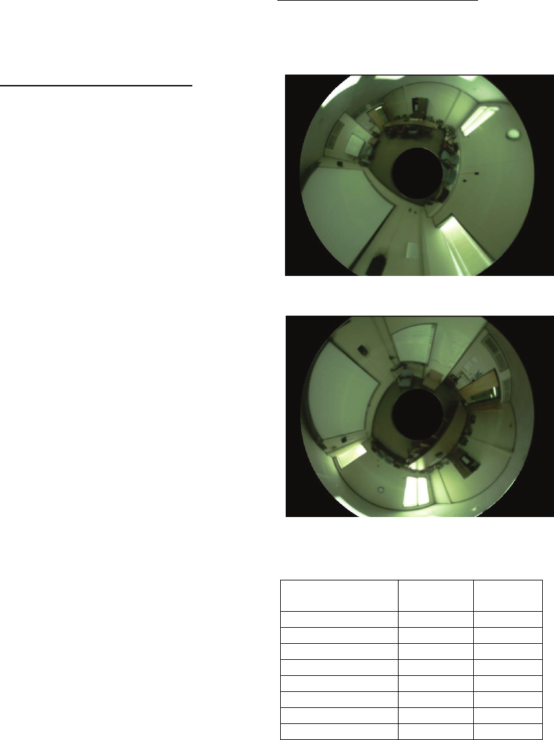
Overall the algorithm did a good job of correctly
identifying the robot’s location. For example, Figure
6 and Figure 7 show a training and test image for
Room 215. The correlation results are given in
Table 1. Additional nodes are given in Tables 2 - 7.
Test Room 215 (Conference Room)
Non-normalized RGB was the only color space that
failed to correctly identify Room 215. However, all
other approaches and color spaces selected the
correct room with a minimum of 73.3% confidence.
Figure 6: Training image for Room 215.
Figure 7: Test image for Room 215.
Table 1: Correlation results for Room 215.
Color Space Node
Selected
%
Confidence
RGB Room 222 73.3
Normalized RGB Room 215 80
HSL Room 215 100
Normalized HSL Room 215 73.3
HSV Room 215 100
Normalized HSV Room 215 80
HSI Room 215 100
Normalized HSI Room 215 73.3

The results from Room 215 illustrate the benefits
of normalizing the color spaces prior to correlation.
In particular, the RGB color space correlation is
improved when normalization of histogram data is
done.
Room 222 (Conference Room)
Room 222 was correctly chosen using all color
spaces with a high degree of confidence.
Figure 8: Test image for Room 222.
Table 2: Correlation results for Room 222.
Color Space Node
Selected
%
Confidence
RGB Room 222 100
Normalized RGB Room 222 93.3
HSL Room 222 100
Normalized HSL Room 222 100
HSV Room 222 100
Normalized HSV Room 222 86.7
HSI Room 222 100
Normalized HSI Room 222 93.3
Room 226A (Small Meeting Room)
Room 226A was correctly chosen using 7 of the
8 color spaces. Again non-normalized RGB was the
single failure.
Figure 9: Test image for Room 226A.
Table 3: Correlation results for Room 226A.
Color Space Node
Selected
%
Confidence
RGB Room 218 60
Normalized RGB Room 226A 66.7
HSL Room 226A 86.7
Normalized HSL Room 226A 73.3
HSV Room 226A 80
Normalized HSV Room 226A 80
HIS Room 226A 80
Normalized HIS Room 226A 86.7
Room 246 (Large Conference Room)
Room 246 was correctly chosen using all color
spaces with a high degree of confidence.
Figure 10: Test image for Room 246.
Table 4: Correlation results for Room 246.
Color Space Node
Selected
%
Confidence
RGB Room 246 86.7
Normalized RGB Room 246 86.7
HSL Room 246 93.3
Normalized HSL Room 246 100
HSV Room 246 93.3
Normalized HSV Room 246 100
HIS Room 246 93.3
Normalized HIS Room 246 100
Sidewalk
The Sidewalk was identified correctly with
86.7% confidence due to the significant color
differences.

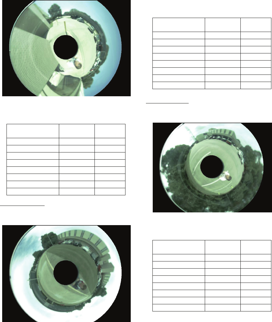
Figure 11: Test image for Sidewalk.
Table 5: Correlation results for Front Sidewalk.
Color Space Node
Selected
%
Confidence
RGB Sidewalk 86.7
Normalized RGB Sidewalk 86.7
HSL Sidewalk 93.3
Normalized HSL Sidewalk 100
HSV Sidewalk 93.3
Normalized HSV Sidewalk 100
HIS Sidewalk 93.3
Normalized HIS Sidewalk 100
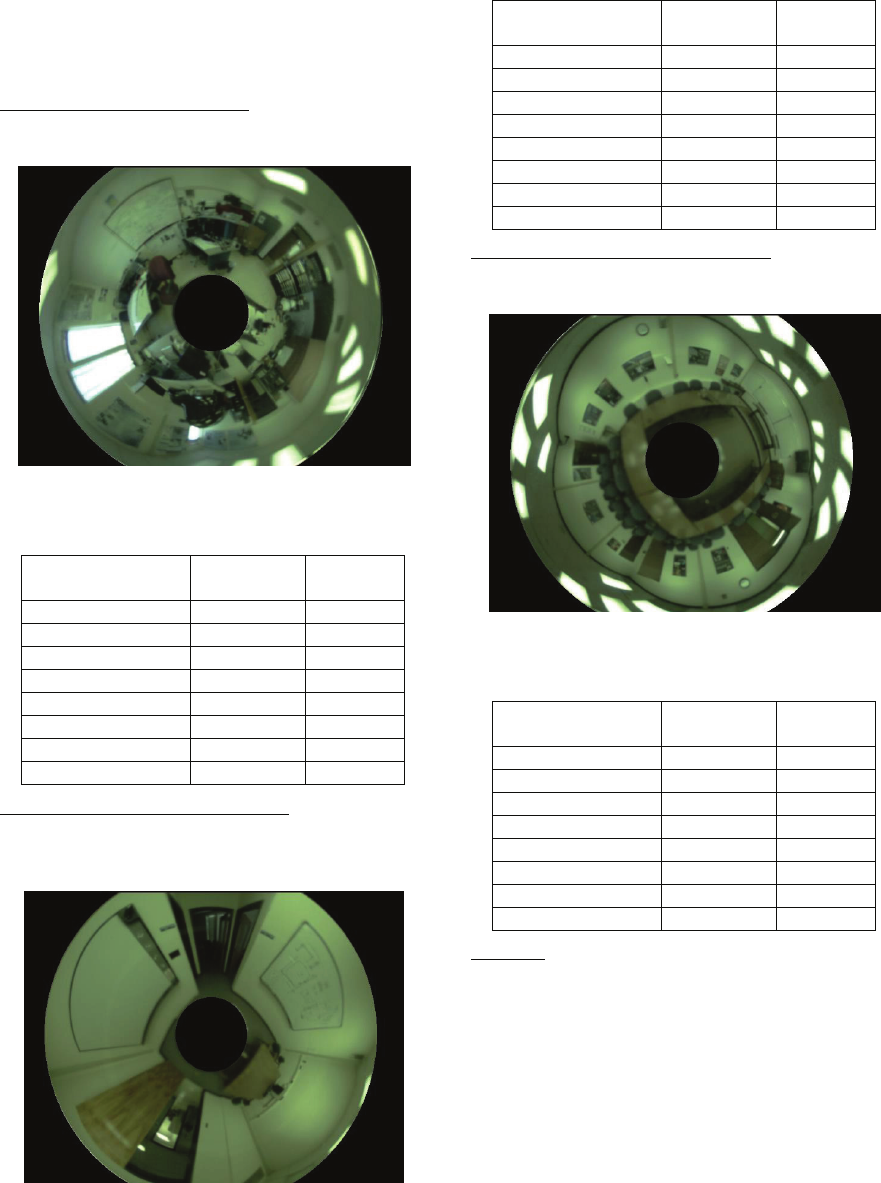
Front Parking Lot
The Front Parking Lot was also easily identified
because of the distinct outdoor color signatures.
Figure 12: Test image for Front Parking Lot.
Table 6: Correlation results for Front Parking Lot.
Color Space Node
Selected
%
Confidence
RGB F. Parking 100
Normalized RGB F. Parking 100
HSL F. Parking 100
Normalized HSL F. Parking 93.3
HSV F. Parking 100
Normalized HSV F. Parking 100
HIS F. Parking 100
Normalized HIS F. Parking 100
Rear Parking Lot
Once again, the Rear Parking Lot was correctly
identified with nearly 100% confidence.
Figure 13: Test image for Rear Parking Lot.
Table 7: Correlation results for Front Parking Lot.
Color Space Node
Selected
%
Confidence
RGB R. Parking 100
Normalized RGB R. Parking 100
HSL R. Parking 100
Normalized HSL R. Parking 93.3
HSV R. Parking 100
Normalized HSV R. Parking 100
HIS R. Parking 100
Normalized HIS R. Parking 100
8 SUMMARY
pIt was demonstrated that color histograms can be
used to perform self-localization, both indoors and
outdoors. Three statistical measures were used to
calculate the distance between training images and
test images. Correlation results from multiple test
and training images across different color spaces

were combined to create a robust correlation
methodology.
Future work will include developing an
autonomous topological mapping system based on
the histogram self-localization algorithm. The
mapping system will allow the robot to identify not
only its current location but also its overall position
in a larger map-based area. Once the robot’s location
is known, adjacency knowledge can be used to do
zone filtering to greatly reduce search sizes.
This sensor-based self-localization could be of
assistance in achieving efficient node-to-node
navigation, path planning, and achieving other
mission objectives.
9 CORRELATION EQUATIONS





,








3

,
(8)



,




∑


·


2






,

∑


·


2






,


3

(9)


,

|




|
3
,
(10)
REFERENCES
Ulrich, I., Nourbakhsh, I. “Appearance-Based Place
Recognization for Topological Localization”, IEEE
International Conference on Robotics and
Automation, April 2000, pp. 1023-1029.
Papoulis, A., Pillai, S. Probability, Random Variable and
Stochastic Processes, New York, NY: McGraw-Hill,
2002, ch. 8.
Abe, Y., Shikano, M., Fukuda, T., Arai, F., and Tanaka,
Y., “Vision Based Navigation System for Autonomous
Mobile Robot with Global Matching”, IEEE
International Conference on Robotics and
Automation, May 1999, pp. 1299-1304.
Kuipers, B.J., “Modeling spatial knowledge,” Cognitive
Science, vol. 2, no. 2, pp. 129-153, 1978.