DIRECTED ACYCLIC GRAPHS AND DISJOINT CHAINS
Yangjun Chen
Dept. Applied Computer Science, University of Winnipeg, Canada
Keywords: Graphs, DAGs, Chains, Paths, Transitive Closure, Reachability Queries.
Abstract: The problem of decomposing a DAG (directed acyclic graph) into a set of disjoint chains has many
applications in data engineering. One of them is the compression of transitive closures to support
reachability queries on whether a given node v in a directed graph G is reachable from another node u
through a path in G. Recently, an interesting algorithm is proposed by Chen et al. (Y. Chen and Y. Chen,
2008) which claims to be able to decompose G into a minimal set of disjoint chains in O(n
2
+ bn
b
) time,
where n is the number of the nodes of G, and b is G’s width, defined to be the size of a largest node subset
U of G such that for every pair of nodes u, v ∈ U, there does not exist a path from u to v or from v to u.
However, in some cases, it fails to do so. In this paper, we analyze this algorithm and show the problem.
More importantly, a new algorithm is discussed, which can always find a minimal set of disjoint chains in
the same time complexity as Chen’s.
1 INTRODUCTION
Given a DAG G(V, E) (directed acyclic graph) with
|V| = n and |E| = e, we want to decompose it into a
minimal set of disjoint chains such that any node in
G appears on some chain, and on each chain, if node
v appears above node u, there is a path from v to u in
G.
This problem is important to compressing a
transitive closure (Wang
et al. , 2006; Warshall, 1962)
to support reachability queries, by which we will
check whether a given node v in G is reachable from
another node u through a path in G (Cohen, 1991;
Cohen
et al., 2003; Cheng et al., 2006; Jagadish,
1990; Schenkel
et al., 2006; Teuhola, 1996; Zibin et
al.
, 2001), which has a wide range of applications.
For example, in object-oriented databases, graph
reachability is important in managing class
inheritance hierarchies.
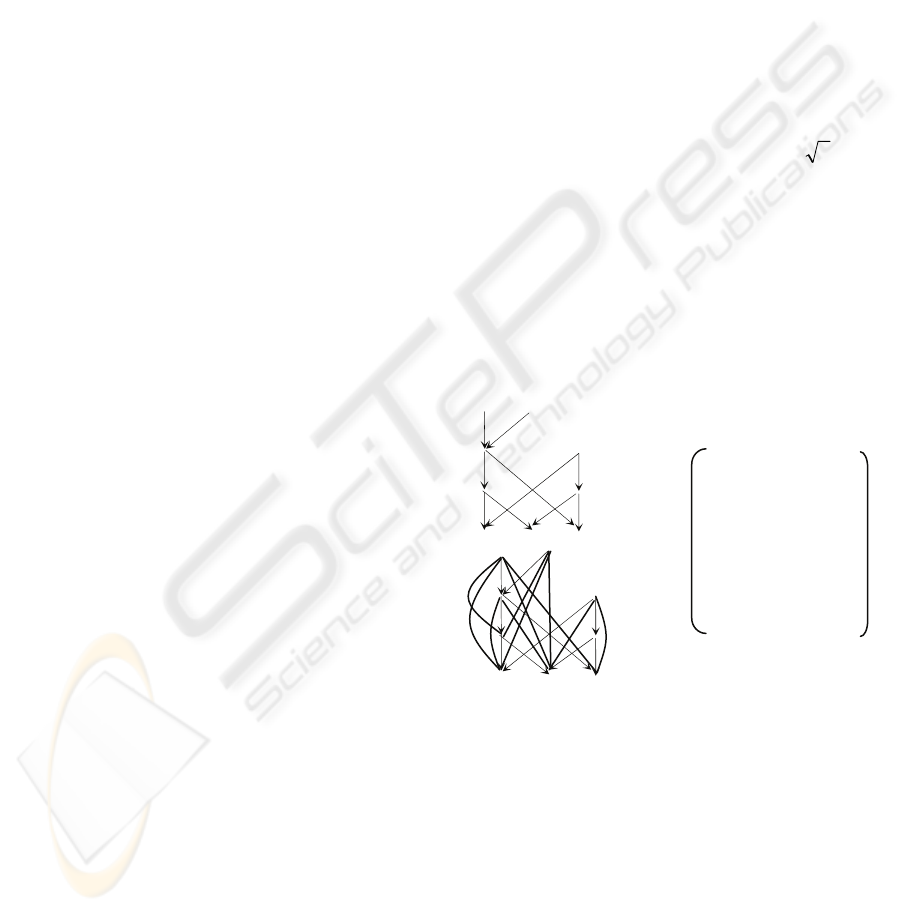
As an example, consider a graph G shown in Fig.
1(a). Its transitive closure is shown in Fig. 1(b). It
can be stored as a 0-1 matrix as shown in Fig. 1(c)
with O(n
2
) space requirement.
Assume that we can decompose G into a set of
disjoint chains as shown in Fig. 2(a). Then, we can
assign each node an index as follows:
(1) Number each chain and number each node on a
chain.
(2) The jth node on the ith chain will be assigned a
pair (i, j) as its index.
Figure 1: DAG, transitive closure and 0-1 matrix.
In addition, each node v on the ith chain will be
associated with an index sequence of length k - 1: (1,
j
1
) … (i – 1, j
i
- 1) (i + 1, j
i
+ 1) … (k, j
k
) such that
any node with index (x, y) is a descendant of v if x =
i and y > j or x ≠ i but y ≥ j
x
, where k is the number
of the disjoint chains. In this way, the space over-
head is decreased to O(kn) (see Fig. 2(a) for
illustration). Especially, we can also store all the
index sequences as a n × k matrix M, in which each
entry M(v, j) is the j-th element in the index
sequence associated with node v. See Fig. 2(b) for
(b)
a b c d e f g h i
1 1 1 1 1 0 0 0 0
0 1 1 1 1 0 0 0 1
0 0 1 1 1 0 0 0 1
0 0 0 1 0 0 0 0 0
0 0 0 0 1 0 0 0 0
0 1 1 1 1 1 0 0 1
0 0 0 1 1 0 1 1 1
0 0 0 0 1 0 0 1 1
0 0 0 0 0 0 0 0 1
a
b
c
d
e
f
g
h
i
(c)
•
•
•
•
•
a
b
c
d
•
•
•
g
h
i
•
f
e
(a)
•
•
•
•
•
a
b
c
d
•
•
•
g
h
i
•
f
e
(b)
17
Chen Y. (2009).
DIRECTED ACYCLIC GRAPHS AND DISJOINT CHAINS.
In Proceedings of the 11th International Conference on Enterprise Information Systems - Databases and Information Systems Integration, pages 17-24
DOI: 10.5220/0001858300170024
Copyright
c
SciTePress

illustration. So, a reachability checking needs only
O(1) time.
Figure 2: Graph encoding.
Note that the above method can also be used for
cyclic graphs (graphs containing cycles) since we
can always transform a cyclic graph to a DAG by
identifying all the strongly connected components
(SCCs) and then collapse each of them into a
representative node. Clearly, all of the nodes in an
SCC is equivalent to its representative as far as
reachability is concerned (Wang
et al., 2006). Using
Tarjan’s algorithm (Tarjan, 1972), all SCCs in G can
be found in O(n + e) time.
This idea was first suggested by Jagadish
(Jagadish, 1991). However, his algorithm needs
O(n
3
) time to decompose a DAG into a minimal set
of disjoint chains (see page 566 in Jagadish, 1991).
For this reason, Jagadish suggested a heuristic
method to decompose a DAG into a set of paths and
then stitch some paths together to form a chain. In
doing so, the number of the produced chains is
normally much larger than the minimum number of
chains, increasing significantly both space and query
time.
In (Y. Chen and Y. Chen, 2008), Chen discussed
a new algorithm to do the task. It requires only O(n
2
+ bn
b
) time, where b is the DAG’s width, defined
to be the size of a largest subset of pairwise unreach-
able nodes. Unfortunately, in some cases, the chain
set found using Chen’s algorithm is not always
minimum.
In this paper, we propose a new algorithm to
decompose a DAG into a minimal set of disjoint
chains. The time complexity of the new algorithm is
still bounded by
O(n
2
+ bn
b
).
The rest of the paper is organized as follows. In
Section 2, we present our algorithm in detail. Then,
in Section 3, we analyze the time complexity.
Finally, a short conclusion is set forth in Section 4.
2 ALGORITHM DESCRIPTION
In this section, we give our new algorithm, which is
inspired by Chen’s algorithm. However, to remove
the problem in Chen’s algorithm, we devise two new
procedures for generating chains and resolving
virtual nodes, respectively.
First, for the chain generation, we distinguish
between two kinds of virtual nodes and handle them
in different ways so that the reachability between
nodes can be transferred bottom-up by using such
virtual nodes.
Second, for the virtual node resolution, a new
data structure, the so-called combined alternating
graph, is constructed so that the number of virtual
nodes resolved at each level is maximized.
In the following, we first discuss how a DAG
can be decomposed into disjoint chains which may
contain virtual nodes in 2.1. Then, in 2.2, we show
how the virtual nodes can be resolved.
2.1 DAG Stratification and Chain
Generation
As with Chen’s algorithm, our algorithm works in
three phases: DAG stratification, chain generation,
and virtual node resolution.
In the first phase, a DAG G(V, E) is stratified
into several levels V
0
, ..., V
h-1
such that V = V
0
∪ ...
∪ V
h-1
and each node in V
i
has its children appearing
only in V
i-1
, ..., V
1
(i = 2, ..., h), where h is the height
of G, i.e., the length of the longest path in G. For
each node v in V
i
, its level is said to be i, denoted l(v)
= i. In addition, C
j
(v) (j < i) represents a set of links
with each pointing to one of v’s children, which
appears in V
j
. Therefore, for each v in V
i
, there exist
i
1
, ..., i
k
(i
l
< i, l = 1, ..., k) such that the set of its
children equals
)(
1
vC
i
∪ ... ∪
)(vC
k
i
. Assume that
V
i
= {v
1
, v
2
, ..., v
l
}. We use
i
j
C
(v) (j < i) to represent
C
j
(v
1
) ∪ ... ∪ C
j
(v
l
).
This phase is almost the same as Chen’s. But for
each node v at a level, we also use B
j
(v) to represent
a set of links with each pointing to one of v’s
parents, which appears in V
j
.
In the second phase, a series of (undirected)
bipartite graphs (Asrtian
et al., 1998; Hopcroft et al.,
1973) will be constructed. In this process, some
virtual nodes may be introduced into the levels V
i
(i
= 1, ..., h - 2). Especially, we distinguish between
two kinds of virtual nodes. One is the virtual nodes
created for actual nodes; and the other is the virtual
nodes generated for virtual nodes. They will be
handled differently.
•
•
•
a
c
e
(1 1)
(2 2)(3 3)
(1 2)
(2 _3)(3, _)
(1, 3)
(2, _)(3, _)
•
•
•
g
h
i
(2, 1)
(1, 2)(3, 3)
(2, 2)
(1, 2)(3, 3)
(2, 3)
(1, _)(3, _)
•
•
•
g
h
i
(3, 1)
(1, _)(2, 3)
(3, 2)
(
1, 3
)(
2,
_)
(3, 3)
(_, _)(2, _)
1 2 3
1 2 3
2 2 3
2 3 -
- 3 -
3 - -
2 1 3
- 3 1
3 - 1
- - 3
a
b
c
d
e
f
g
h
i
a chain
(a) (b)
ICEIS 2009 - International Conference on Enterprise Information Systems
18
In the following, we begin our discussion with a
summarization of some important concepts related
to bipartite graphs, which are needed to define
virtual nodes.
Definition 1. (concepts related to matching, Asrtian
et al., 1998) Let G(V, E) be a bipartite graph. Let M
be a maximum matching of G. A node v is said to be
covered by M, if some edge of M is incident to v.
We will also call an uncovered node free. A path or
cycle is alternating, relative to M, if its edges are
alternately in E\M and M. A path is an augmenting
path if it is an alternating path with free origin and
terminus.
In addition, it is well known that using the
Hopcroft-Karp algorithm (Hopcroft
et al., 1973) a
maximum matching of G can be found in
O(|E|
||V
) time.
Also, the following symbols are used for ease of
explanation:
V
i
’ = V
i
∪ {virtual nodes introduced into V
i
}.
C
i
= (v) ∪ {all the new edges from the nodes in V
i
to the virtual nodes introduced into V
i-1
}
G(V
i
, V
i-1
’; C
i
) - the bipartite graph containing V
i
and
V
i-1
’.
Definition 2. (virtual nodes for actual nodes) Let
G(V, E) be a DAG, divided into V
0
, ..., V
h-1
(i.e., V =
V
0
∪ ... ∪ V
h-1
). Let M
i
be a maximum matching of
the bipartite graph G(V
i
, V
i-1
’; C
i
) and v be a free
actual node (in V
i-1
’) relative to M
i
(i = 1, ..., h - 1).
Add a virtual node v’ into V
i
. In addition, for each
node u ∈ V
i+1
, a new edge u → v’ will be created if
one of the following two conditions is satisfied:
1. u → v ∈ E; or
2. There exists an edge (v
1
, v
2
) covered by M
i
such
that v
1
and v are connected through an alternating
path relative to M
i
; and u ∈ B
i+1
(v
1
) or u ∈
B
i+1
(v
2
).
v is called the source of v’, denoted s(v’).
A virtual edge from v’ to v is also generated to
indicate the relationship between v and v’. Besides, a
new edge u → v’ will be marked with ‘directly
connectable’ if one of the following conditions are
satisfied:
1. u → v ∈ E; or
2. There is an alternating path of length 1, which
connects v
1
and v. That is, v
1
→ v ∈ E.
We mark these edges with ‘directly connectable’
because it is possible for us to directly connect u and
v to remove v’.
The following example helps for illustration.
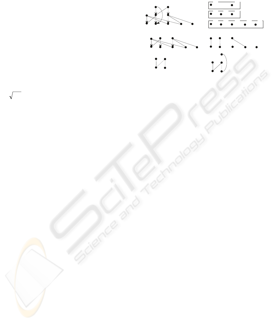
Example 1. Consider the graph shown in Fig. 3(a).
It can be divided into three levels as shown in Fig.
3(b). The bipartite graph made up of V
1
and V
0
,
G(V
1
, V
0
; C
1
), is shown in Fig. 3(c) and a possible
maximum matching M
1
of it is shown in Fig. 3(d).
Figure 3: A bipartite graph and a maximum matching.
Relative to M
1
, we have two free nodes i and a. For
them, two virtual nodes i’ and a’ will be constructed.
Then, V
1
’ = {b, e, h, i’, a’}. In addition, four new
edges (d, i’), (d, a’), (g, i’), and (g, a’) will be
constructed. But all of them will not be marked with
‘directly connectable’.
The motivation of constructing such a virtual
node (e.g., i’) is that it is possible to connect f to d or
g to form part of a chain if we transfer the edges on
an alternating path: b → c → e → f (see Fig. 3(e),
where a solid edge represents an edge belonging to
M
1
while a dashed edge to C
1
\M
1
), or h → j → b → c
→ e → f. Then, we can connect d or g to f, as well as
b or h to i without increasing the number of chains,
as illustrated in Fig. 3(f). This can be achieved by
the virtual node resolution process (see 2.2).
For the graph shown in Fig. 4(a), which is the
second bipartite graph established for the graph
shown in Fig. 3.4(a), a possible maximum matching
M
2
is shown in Fig. 4(b). So M
1
∪ M
2
is a set of
chains as shown in Fig. 4(c)
Definition 3. (virtual nodes for virtual nodes) Let M
i
be a maximum matching of the bipartite graph G(V
i
,
V
i-1
’; C
i
) and v’ be a free virtual node (in V
i-1
’)
relative to M
i
(i = 1, ..., h - 1). Add a virtual node v’’
into V
i
. Set s(v’’) to be w = s(v’). Let l(w) = j. For
each node u ∈ V
i+1
, a new edge u → v’ will be
created if there exists an edge (v
1
, v
2
) covered by
M
j+1
such that v
1
and w are connected through an
alternating path relative to M
j+1
; and u ∈ B
i+1
(v
1
) or u
∈ B
i+1
(v
2
).
Again, a virtual edge from v’’ to v’ will be
generated to facilitate the virtual node resolution
process.
(a)
b
ac
g
h
i
f
e
d
j
ac i
f
j
b h
e
d
g
V
0
:
V
1
:
V
2
:
(b)
b
ac
h
i
f
e
j
V
0
:
V
1
:
a
h
i
e
b
c
f
j
b
c
f
e
g
b
c
f
e
(c) (d)
(e) (f)
DIRECTED ACYCLIC GRAPHS AND DISJOINT CHAINS
19
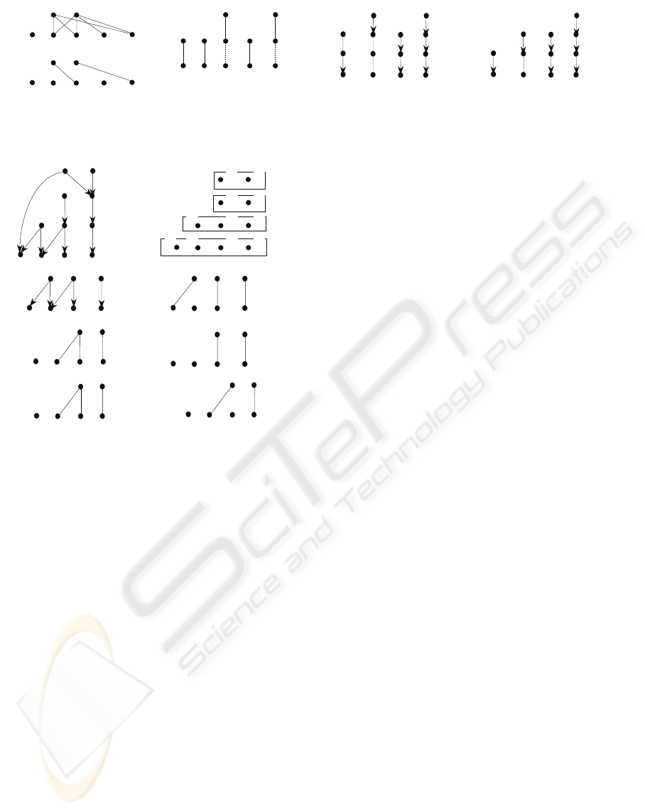
Figure 4: A bipartite graph and a maximum matching.
Example 2. Consider the graph shown in Fig. 5(a).
Figure 5: Illustration for virtual nodes.
This graph can be divided into four levels as
shown in Fig. 5(b). The first bipartite graph
consisting of V
1
and V
0
, G(V
1
, V
0
; C
1
), is shown in
Fig. 5(c) and a possible maximum matching M
1
of it
is shown in Fig. 5(d). Relative to M
1
, we have a free
node f. For it, a virtual nodes f’ will be constructed.
Then, V
1
’ = {b, f’, d, h} (see Fig. 5(e)). Assume that
the maximum matching found for G(V
2
, V
1
’; C
2
) is
as shown in Fig. 5(f). A virtual node f’’ for f’ will be
established. So V
2
’ = {f’’, e, g}. Especially, we are
able to connect node f’’ and node p for the following
reason:
i) s(f’’) = s(f’) = f;
ii) (b, c) ∈ M
1
;
iii) f is connected to b through an alternating path: f
→ b; and
iv) p ∈ B
3
(c).
The corresponding bipartite graph G(V
3
, V
2
’; C
3
)
is shown in Fig. 5(g). The unique maximum
matching of G(V
3
, V
2
’; C
3
) is shown in Fig. 5(h).
By unifying M
1
, M
2
, and M
3
, we get a set of disjoint
chains as shown in Fig. 6(a).
Figure 6: Illustration for disjoint chains.
2.2 Virtual Node Resolution
In the third phase, we will remove all the virtual
nodes. This will be done top-down level by level;
and at each level any virtual node, which does not
have a parent along a chain, will be simply
eliminated. In addition, we call a virtual node v’ a
transit virtual node if one of the following two
conditions is satisfied.
1. Let u, v’, w be three consecutive nodes on a chain.
u → v’ is a marked edge (i.e., a directly
connectable edge); or
2. w is a virtual node.
In both cases, we connect u and w and then
remove v’. It is because in case (1), both u and w are
actual nodes and we have u → w ∈ E or there exists
a actual node x such that u → x ∈ E and x → w ∈ E.
In case (2), w is a virtual node, working as a
‘transfer’ of reachability.
For example, since node f’ in Fig. 6(a) is a
virtual node, node f’’ is a transit virtual node. It can
be directly removed, leading to a set of chains as
shown in Fig. 6(b). But node f’ cannot be removed
in this way since it is not a transit virtual node.
In the following, we discuss how to resolve a non-
transit virtual node, for which more effort is needed.
First, we define a new concept.
Definition 4. (alternating graph) Let M
i
be a
maximum matching of G(V
i
, V
i-1
’; C
i
). The
alternating graph
i
G
G
with respect to M
i
is a directed
graph with the following sets of nodes and edges:
V(
i
G
G
) = V
i
∪ V
i-1
’, and
E(
i
G
G
) = {u → v | u ∈ V
i-1
’, v ∈ Vi, and (u, v) ∈ M
i
}
∪ {v → u | u ∈ V
i-1
’, v ∈ V
i
, and (u, v) ∈ C
i
\M
i
}.
Example 3. Consider the graph shown in Fig. 3(a)
once again. Relative to M
1
of G(V
1
, V
0
; C
1
) shown in
Fig. 3(d), nodes i and a are two free nodes. The
alternating graph with respect to M
1
is shown in Fig.
7(a). It is redrawn in Fig. 7(b) for a clear
explanation.
In order to resolve the non-transit virtual nodes
in V
i
’, we will combine
1+
i
G
G
and
i
G
G
by connecting
(a) (b)
i
d
e
k
h
g
q
f
f’
f
’
’
p
c
b
b’
i
d
e
k
h
g
q
f
f’
p
c
b
(a)
c
i
f
k
d
b
h
e
g
p
q
(d)
c
i
f
k
d
b
h
M
1
:
(b)
(c)
c
i
f
k
d
b
h
V
0
:
V
1
:
(e)
b
d
f’
h
e
g
V
1
’:
V
2
:
(f)
b
d
f’
h
e
g
M
2
:
(g)
b
e
f
’
’
g
p
q
V
2
’:
V
3
:
(h)
b
e
f
’
’
g
p
q
M
3
:
V
2
:
V
3
:
p
q
e
g
d
b
h
V
0
:
V
1
:
c
i
f
k
(a)
(b) (c)
V
1
’:
V
2
:
b
g
i’
e
d
h
a’
b
g
i’
e
d
h
a’
c i
f
j
a
b i’
e
h a’
d
g
ICEIS 2009 - International Conference on Enterprise Information Systems
20

some nodes v’ in
1+
i
G
G
to some nodes u in
i
G
G
if the
following conditions are satisfied.
(i) v’ is a non-transit virtual node appearing in V
i
’.
(Note that V(
1+
i
G
G
) = V
i+1
∪ V
i
’.)
(ii) There exist a node x in V
i+1
and a node y in V
i
such that (x, v’) ∈ M
i+1
, x → y ∈ C
i+1
, and (y, u)
∈ M
i
.
We denote this combined graph by
1+
i
G
G
⊕
i
G
G
.
Figure 7: An alternating graph.
For illustration, consider G(V
2
, V
1
’; C
2
) shown in
Fig. 4(a). Assume that the found maximum matching
M
2
is as shown in Fig. 4(b). Then, the alternating
graph
2
G
G
(with respect to M
2
) is a graph shown in
Fig. 8(a).
2
G
G
⊕
1
G
G
is shown in Fig. 8(b). Note that
i’ and a’ are two non-transit virtual nodes.
Figure 8: Illustration for combined graph.
We also remark that a node in
1+
i
G
G
and a node in
i
G
G
may share the same node name. But they will be
handled as different nodes. For example, node e in
2
G
G
and node e in
1
G
G
are different.
In Fig. 8(b), we connect node a’ (in
2
G
G
) to node f
(in
1
G
G
) for the following reason.
(1) a’ is a non-transit virtual node introduced into
V
1
.
(2) (g, a’) ∈ M
2
, g → e ∈ C
2
, and (e, f) ∈ M
1
.
As mentioned above, we connect a’ to f since it
is possible for us to transfer the edges on an
alternating path (relative to M
1
) starting from node f
(relative to M
1
) and terminating at free node i or a
(in V
0
), which will make i or a covered without in-
creasing the number of chains.
The same analysis applies to node i’ (in
2
G
G
),
which is also connected to node f (in
1
G
G
).
In order to resolve as many non-transit virtual nodes
(appearing in V
i
’) as possible, we need to find a
maximum set of node-disjoint paths (i.e., no two of
these paths share any nodes), each starting at a non-
transit virtual node (in
1+
i
G
G
) and ending at a free
node in
1+
i
G
G
, or ending at a free node in
i
G
G
. For
example, to resolve a’ and i’, we need first to find
two paths in the above combined graph, as shown in
Fig. 9(a).
Figure 9: Illustration for node-disjoint paths.
(In Fig. 9(b), we show another two node-disjoint
paths.)
By transferring the edges on such a path, the
corresponding virtual node can be removed as
follows.
(1) Let v
1
→ v
2
→ ... → v
k
be a found path. Transfer
the edges on the path.
(2) If v
k
is a node in
1+
i
G
G
, we simply remove the
corresponding virtual node v
1
.
(3) If v
k
is a node in
i
G
G
, connect the parent of v
1
along the corresponding chain to v
2
. Remove v
1
.
For instance, by transferring the edges on the path
from a’ to e (in
2
G
G
) in Fig. 9(a), we will connect g
to e (in
2
G
G
). a’ will be removed. By transferring the
edges on the path from i’ to a in Fig. 9(a), we will
connect h (in
1
G
G
) to a, b to j, e to c, and d to f. Then,
i’ is removed. Note that a is in
1
G
G
and d is the parent
of i’ along a chain (see Fig. 4(c)). In this way, we
will change the chains shown in Fig. 4(c) to the
chains shown in Fig. 10(a) with all the virtual nodes
being removed. The number of chains is still 5.
By resolving node f’ in the chain set shown in Fig.
6(b), we will get a set of disjoint chains shown in
Fig. 10(b).
Figure 10: Minimum sets of chains.
(a)
c i
f
j
a
b
e
h
d
g
c
i
f
k
d b
h
e
g
p
q
(b)
(a)
(b)
f
e c b
j
h a
a’
g
e
i
f
e c b
a’
g
i’
i’
b
ac
h
i
f
e
j
V
0
:
V
1
:
(a)
i
f
e c b
j
h
a
(b)
DIRECTED ACYCLIC GRAPHS AND DISJOINT CHAINS
21

It remains to show how to find a maximal set of
node-disjoint paths in
1+
i
G
G
⊕
i
G
G
.
For this purpose, we define a maximum flow
problem over
1+
i
G
G
⊕
i
G
G
(with multiple sources and
sinks) as follows.
1) Each non-transit virtual node in
1+
i
G
G
is
designated as a source. Each free node (in
1+
i
G
G
)
relative to M
i+1
, or free node (in
i
G
G
) relative to M
i
is designated as a sink.
2) Each edge u → v is associated with a capacity
c(u, v) = 1. (If (u, v) is not an edge in
1+
i
G
G
⊕
i
G
G
,
c(u, v) = 0.)
Generally, to find a maximum flow in a network,
we need O(n
3
) time (Even, 1979; Karzanov, 1974;
Cotman et al., 2001). However, a network as
constructed above is a 0-1 network. In addition, for
each node v, we have either d
in
(v) ≤ 1 or d
out
(v) ≤ 1,
where d
in
(v) and d
out
(v) represent the indegree and
outdegree of v in
1+
i
G
G
⊕
i
G
G
, respectively. It is
because each path in
1+
i
G
G
⊕
i
G
G
is an alternating path
relative to M
i+1
or relative to M
i
. So each node
excerpt sources and sinks is an end node of an edge
covered by M
i+1
or by M
i
. As shown in (Even, 1979,
Theorem 6.3 on page 120), it needs only O(
n
e)
time to find a maximum flow in this kind of
networks. Especially, a maximum flow exactly
corresponds to a maximal set of disjoint paths. See
the proof of Lemma 6.4 in (Even, 1979, page 120.)
According to the above discussion, we give the
following algorithm for resolving virtual nodes. We
assume that each virtual node has a parent along a
chain. Otherwise, it can be simply eliminated.
Algorithm virtual-resolution(S)
input: S - a chain set obtained by executing the chain
generation process.
output: a set of chains containing no virtual nodes.
begin
1. for i = h - 2 downto 1 do
2. {for any transit virtual node v’ in V
i
’ do
3. {
4. let u, v’, w be three consecutive nodes on a
chain;
5. connect u and w;
6. }
7. construct
1+
i
G
G
⊕
i
G
G
; (*Begin to handle
non-transit virtual nodes.*)
8. find a maximal
set of node disjoint paths: P
1
, ... P
l
;
9. for j = 1 to l do
10. {let P
j
= v
1
→ v
2
→ ... → v
k
;
11. if v
k
is a free node relative to M
i
then
12. {transfer the edges on P
j
; remove v
1
;}
13. else (* v
k
is a free node relative to M
i-1
.*)
14. {let u be a node such that (u, v
1
) ∈ M
i
;
15. transfer the edges on P
j
; remove v
1
;
16. connect u to v
2
;
17. }
18. removed any unsolved virtual node;
19. }
end
In the main for-loop of the above algorithm, we
first handle transit virtual nodes (lines 2 - 6). Then,
we construct
i
G
G
⊕
1−
i
G
G
to resolve all the non-transit
virtual nodes (see line 7.) For this purpose, we
search for a maximal set of node disjoint paths (see
line 8). We also distinguish between two kinds of
node disjoint paths: paths ending at a free node
relative to M
i
, and paths ending at a free node
relative to M
i-1
. For the first kind of paths, we simply
transfer the edges on a path and then remove the
corresponding virtual node (see line 12). For the
second kind of paths, we need to do something more
to connect the parent of the corresponding virtual
node (along the chain) to the second node of the path
(see line 16). In line 18, we remove all those virtual
nodes, which cannot be resolved. Each of such
virtual nodes leads to splitting of a chain into two
chains.
Note that removing a transit virtual node will not
increase the number of chains. Also, resolving a
non-transit virtual node using a node disjoint path
does not lead to a chain splitting. So the number of
increased chains during the virtual node resolution
process is minimum since the number of node
disjoint paths is maximum.
3 TIME COMPLEXITY
Now we analyze the computational complexities of
our algorithm. The cost of the whole process can be
divided into three parts:
- cost
1
: the time for stratifying a DAG.
- cost
2
: the time for generating disjoint chains,
which may contain virtual nodes.
- cost
3
: the time for resolving virtual nodes.
As shown in (Chen and Chen, 2008), cost
1
is
bounded by O(n + e).
cost
2
mainly contains two parts. One part: cost
21
is the time for finding a maximum matching of every
G(V
i
, V
i-1
’; C
i
) (i = 1, ..., h - 1; V
0
’ = V
0
). The other
part: cost
22
is the time for checking whether, for each
actual free node appearing in V
i-1
’, there exists an
ICEIS 2009 - International Conference on Enterprise Information Systems
22
edge (v
1
, v
2
) covered by M
i
such that v
1
and v are
connected through an alternating path relative to M
i
.
The time for finding a maximum matching of G(V
i
,
V
i-1
’; C
i
) is bounded by
O(
'
1−
+
ii
VV
· | C
i
’|). (see Chen et al., 2008)
Therefore, cost
21
is bounded by
O(
∑
−
=
−
⋅+
1
1
1
|'|||
h
i
ii
VV
|C
i
’|)
≤ O(
∑
−
=
⋅
1
1
||
h
i
i
Vbb
) = O(b
b
n).
cost
22
can be analyzed as follows. We construct a
small boolean n
i
× m
i
matrix A
i
, where n
i
is the
number of free actual nodes in V
i-1
and m
i
is the
number of all the covered actual nodes in V
i
. Each
entry a
jk
= 1 in A
i
indicates that there exists an
alternating path (relative to M
i
) connects node j and
k. Using the algorithm discussed in (Coppersmith et
al., 1990) for matrix multiplication, cost
22
can be
estimated by
Ο(
∑
−
=
−
+
1
1
376.2
1
|)||(|
h
i
ii
VV
)
= Ο(
376.0
1
1
1
2
1
2
1
|)||)(|||||||2|(|
ii
h
i
iiii
VVVVVV +++
−
−
=
−−
∑
)
≤ O(
∑
−
=
⋅
1
1
||
h
i
i
Vbb
) = O(b
b
n).
During the virtual-resolution process, the virtual
nodes are resolved level by level. At each level, the
number of the nodes in
i
G
G
⊕
1−
i
G
G
is bounded by
O(|V
i+1
| + 2|V
i
’| + |V
i-1
’|); and the number of its edge
is O(|C
i
| + |C
i-1
|). So, the time for finding a maximal
set of node-disjoint paths in
i
G
G
⊕
1−
i
G
G
is bounded
by O(
|'||'|2|
11 −+
++
iii
VVV
(|C
i
| + |C
i-1
|)). So the
total cost of the virtual node resolution is in the
order of
∑
−
=
−+
++
1
2
11
|'||'|2|'|
h
i
iii
VVV
· (|C
i
| + |C
i-1
|).
= O(
∑
−
=
⋅
1
1
||
h
i
i
Vbb
) = O(b
b
n).
From the above analysis, we get the following
proposition.
Proposition 1. The time complexity of the whole
process to decompose a DAG into a minimized set
of disjoint chains is bounded by O(bn
b
).
The space complexity of the whole process is
bounded by O(e + bn) since the number of the newly
added edges in each bipartite graph G(V
i
, V
i-1
’; C
i
’)
is bounded by O(b|V
i-1
|), and the size of each matrix
A
i
is bounded by O(|V
i-1
|
2
).
4 CONCLUSIONS
In this paper, a new algorithm for resolving virtual
nodes is discussed, which is a critic step in an
algorithm proposed by Chen
et al. (Chen and Chen,
2008) to decompose a DAG into a set of disjoint
chains. In addition, the virtual node resolution
process of Chen’s algorithm is analyzed, showing
that in some cases Chen’s algorithm fails to find a
minimal set of disjoint chains. The main idea of our
algorithm is the construction of alternating graphs.
By finding a maximal set of node disjoint paths in
such a graph to resolve virtual nodes, we are able to
guarantee that at each step of virtual node resolution,
the number of increased chains is minimum.
REFERENCES
H. Alt, N. Blum, K. Mehlhorn, and M. Paul, Computing a
maximum cardinality matching in a bipartite graph in
time O(n
1.5
), Information Processing Letters,
37(1991), 237 -240.
A. S. Asratian, T. Denley, and R. Haggkvist, Bipartite
Graphs and their Applications, Cambridge University,
1998.
J. Banerjee, W. Kim, S. Kim and J.F. Garza, "Clustering a
DAG for CAD Databases," IEEE Trans. on Knowl-
edge and Data Engineering, Vol. 14, No. 11, Nov.
1988, pp. 1684-1699.
K. S. Booth and G.S. Leuker, “Testing for the consecutive
ones property, interval graphs, and graph planarity
using PQ-tree algorithms,” J. Comput. Sys. Sci.,
13(3):335-379, Dec. 1976.
Y. Chen and Y. Chen, An Efficient Algorithm for An-
swering Graph Reachability Queries, Proceedings of
ICDE, 2008, pp. 893 - 902.
Y. Chen, “On the Graph Traversal and Linear Binary-
chain Programs,” IEEE Transactions on Knowledge
and Data Engineering, Vol. 15, No. 3, May 2003, pp.
573-596.
N. H. Cohen, “Type-extension tests can be performed in
constant time,” ACM Transactions on Programming
Languages and Systems, 13:626-629, 1991.
E. Cohen, E. Halperin, H. Kaplan, and U. Zwick,
Reachability and distance queries via 2-hop labels,
SIAM J. Comput, vol. 32, No. 5, pp. 1338-1355, 2003.
J. Cheng, J.X. Yu, X. Lin, H. Wang, and P.S. Yu, Fast
computation of reachability labeling for large graphs,
in Proc. EDBT, Munich, Germany, May 26-31, 2006.
D. Coppersmith, and S. Winograd. Matrix multiplication
via arithmetic progression. Journal of Symbolic
Computation, vol. 9, pp. 251-280, 1990.
DIRECTED ACYCLIC GRAPHS AND DISJOINT CHAINS
23

R. P. Dilworth, A decomposition theorem for partially
ordered sets, Ann. Math. 51 (1950), pp. 161-166.
S. Even, Graph Algorithms, Computer Science Press, Inc.,
Rockville, Maryland, 1979.
J. E. Hopcroft, and R.M. Karp, An n2.5 algorithm for
maximum matching in bipartite graphs, SIAM J. Com-
put. 2(1973), 225-231.
H. V. Jagadish, "A Compression Technique to Materialize
Transitive Closure," ACM Trans. Database Systems,
Vol. 15, No. 4, 1990, pp. 558 - 598.
A. V. Karzanov, Determining the Maximal Flow in a
Network by the Method of Preflow, Soviet Math.
Dokl., Vol. 15, 1974, pp. 434-437.
T. Keller, G. Graefe and D. Maier, "Efficient Assembly of
Complex Objects," Proc. ACM SIGMOD Conf., Den-
ver, Colo., 1991, pp. 148-157.
H. A. Kuno and E.A. Rundensteiner, "Incremental
Maintenance of Materialized Object-Oriented Views
in MultiView: Strategies and Performance
Evaluation," IEEE Transactions on Knowledge and
Data Engineering, vol. 10. No. 5, 1998, pp. 768-792.
T. Cotman, C. Leiserson, R. Rivest, and C. Stein, Intro-
duction to Algorithms (second edition), McGraw-Hill
Book Company, Boston, 2001.
R. Schenkel, A. Theobald, and G. Weikum, Efficient
creation and incrementation maintenance of HOPI in-
dex for complex xml document collection, in Proc.
ICDE, 2006.
R. Tarjan: Depth-first Search and Linear Graph Algo-
rithms, SIAM J. Compt. Vol. 1. No. 2. June 1972, pp.
146 -140.
J. Teuhola, "Path Signatures: A Way to Speed up Recur-
sion in Relational Databases," IEEE Trans. on Knowl-
edge and Data Engineering, Vol. 8, No. 3, June 1996,
pp. 446 - 454.
H. S. Warren, “A Modification of Warshall’s Algorithm
for the Transitive Closure of Binary Relations,” Com-
mun. ACM 18, 4 (April 1975), 218 - 220.
H. Wang, H. He, J. Yang, P.S. Yu, and J. X. Yu, Dual La-
beling: Answering Graph Reachability Queries in
Constant time, in Proc. of Int. Conf. on Data
Engineering, Atlanta, USA, April -8 2006.
S. Warshall, “A Theorem on Boolean Matrices,” JACM, 9.
1(Jan. 1962), 11 - 12.
Y. Zibin and J. Gil, "Efficient Subtyping Tests with PQ-
Encoding," Proc. of the 2001 ACM SIGPLAN Conf. on
Object-Oriented Programming Systems, Languages
and Application, Florida, October 14-18, 2001, pp. 96-
107.
ICEIS 2009 - International Conference on Enterprise Information Systems
24
