INTELLIGENT SURVEILLANCE FOR TRAJECTORY ANALYSIS
Detecting Anomalous Situations in Monitored Environments
J. Albusac
Escuela Universitaria Politecnica de Almaden, University of Castilla-La Mancha
c/Plaza Manuel Meca 1, Almaden, Spain
J. J. Castro-Schez, L. Jimenez-Linares, D. Vallejo, L. M. Lopez-Lopez
Escuela Superior de Informatica, University of Castilla-La Mancha, c/Paseo de la Universidad 4, Ciudad Real, Spain
Keywords:
Artificial Intelligent, Surveillance Systems, Image Understanding, Normality Analysis.
Abstract:
Recently, there is a growing interest in the development and deployment of intelligent surveillance systems
capable of finding out and analyzing simple and complex events that take place on scenes monitored by
cameras. Within this context, the use of expert knowledge may offer a realistic solution when dealing with the
design of a surveillance system. In this paper, we briefly describe the architecture of an intelligent surveillance
system based on normality components and expert knowledge. These components specify how a certain object
must ideally behave according to one concept. A specific normality component which analyzes the trajectories
followed by objects is studied in depth in order to analyze behaviors in an outdoor environment. The analysis
of trajectories in the surveillance context is an interesting issue because any moving object has always a goal
in an environment, and it usually goes towards one destination to achieve it.
1 INTRODUCTION
In the last few years, many researchers have proposed
many models and techniques for event and behav-
ior understanding. Thanks to these proposals many
software prototypes and systems have been developed
and tested over real scenes, VSAM (Collins et al.,
2000), W4 (Haritaoglu et al., 2000), (Hudelot and
Thonnat, 2003) or (Bauckhage et al., 2004). In spite
of these advances, there is a long way to achieve ro-
bust systems capable of interpreting a scene with the
same precision as human beings do.
To face this challenge, it is necessary to design
a complete surveillance system consisting of differ-
ent layers (Wang and Maybank, 2004). Some of
these layers could be as follows: (i) environment
modelling to provide the system with the knowledge
needed to carry out surveillance, (ii) segmentation
and tracking of objects, (iii) multimodal sensor fusion
and event and behavior understanding, (iv) decision-
making and crisis management and, finally, (v) multi-
media content-based retrieval layer to perform foren-
sic analysis. Every layer implies a wide field of inves-
tigation and, for this reason, most researchers focus
their work on one of these layers.
Middle layers aims at analyzing complex behav-
iors from information obtained by low-level sensors.
In fact, a complex behavior is a sequence of simple
events that are temporaly related. Moreover, these
layers must also be capable of dealing with uncer-
tainty and imprecision inherent in real world prob-
lems, that is, an artificial surveillance system, in most
cases, is not able to absolutely determine what is hap-
pening in a concrete instant. To carry out surveillance,
several types of analysis can be made to determine
normality in monitored environments. For instance,
trajectory analysis, speed study, proximity relation-
ships among objects, suspicious objects, access con-
trol, etc.
In any environment, every moving object has a
goal and it usually goes towards one destination to
achieve it (Dee and Hogg, 2004). For this reason,
the analysis of trajectories followed by objects is in-
teresting to detect anomalies in monitored environ-
ments. Several authors have addressed this issue in
the literature. (Johnson and Hogg, 1996) proposed a
statistically based model for learning object trajecto-
ries in monitored environments. Learned trajectories
are represented by the distribution of prototype vec-
tors using neuronal networks and vector quantisation.
102
Albusac J., Castro-Schez J., Jimenez-Linares L., Vallejo D. and Lopez-Lopez L. (2009).
INTELLIGENT SURVEILLANCE FOR TRAJECTORY ANALYSIS - Detecting Anomalous Situations in Monitored Environments.
In Proceedings of the 11th International Conference on Enterprise Information Systems - Artificial Intelligence and Decision Support Systems, pages
103-108
DOI: 10.5220/0001953901030108
Copyright
c
 SciTePress

(Makris and Ellis, 2002) also proposed a model for
extracting pedestrian trajectories in outdoors environ-
ments. In this model, paths are described by means of
entry/exit zones and junctions (regions where routes
cross each other). (Piciarelli et al., 2005) discussed a
trajectory clustering method suited for video surveil-
lance and monitoring systems. One great advantage
of this method is its capacity for dynamically build-
ing clusters in real-time.
In contrast to these works, we address trajectory
analysis from a more general point of view. Our
definition of the trajectory concept is based on re-
strictions, which allow us to not only define trajec-
tories but also who or when moving objects can fol-
low them. In fact, flexibility and generality are two
key issues when designing surveillance systems. This
way, the model proposed in this paper lets expand the
concept to be analyzed with new restrictions when
needed.
In this paper, we propose a surveillance system
based on normality components. The global normal-
ity analysis in an environment is given from the unifi-
cation of partial analysis offered for each component.
One of these components aims at analyzing trajecto-
ries followed by objects and deals with uncertainty
and imprecision by means of the fuzzy logic theory
(Zadeh, 1996). Fuzzy logic allows us to easily work
with uncertainty and to deploy a relatively simple sys-
tem with short response times.
The rest of this paper is organized in the follow-
ing way. Section 2 describes the architecture of the
intelligent surveillance system. This system includes
a module that analyzes the trajectories followed by
objects. Section 3 discusses in detail the trajectory
normality component. In Section 4, we show how
this component works in a real environment through
a case study. Finally, Section 5 concludes the paper
and suggests future research lines.
2 DESCRIPTION OF THE
SYSTEM ARCHITECTURE
The architecture of our surveillance system (OCU-
LUS) consists of three main layers. Layer 0 refers to
the perceptual layer, that is, the information retrieval
from the environment by means of different sensors.
Such information can be directly sent to the upper
layer (e.g. presence sensors) or processed in order
to obtain the required data (e.g. video or audio). It is
important to remark that most of this information is
surrounded by uncertainty and vagueness and, there-
fore, our model deals with this handicap from the per-
ceptual layer.
Layer 1 refers to the conceptual layer that covers
all the mechanisms for normality analysis. Interac-
tions with Layer 0 involve the set of input variables
(V) used to analyze the environment normality and
the set of domain definitions (DDV) of such variables.
Each normality component is responsible for analyz-
ing the normality about a concrete concept. OCULUS
makes possible to dinamically add or remove compo-
nents. For example, if we require to add a normality
concept about correct accesses, OCULUS allows to
directly plug it in. Due to the inherently distributed
nature of surveillance and the different components of
the architecture, a multi-agent system has been used
to support OCULUS. There are different agents spe-
cialized into each one of the normality concepts de-
ployed. When an agent is instantiated into the agent
platform, it automatically loads the knowledge about
the normality component required. Currently, we are
using CLIPS for representing such knowledge and for
making the reasoning process and the middleware Ze-
roC ICE (Henning, 2004) for carrying out communi-
cation among agents.
Finally, Layer 2 refers to crisis management and
decision making processes. The information used by
this layer depends on the analysis of Layer 1, which
may come from three modules defined on top of Layer
1: i) identification of anomalous situations, that is,
what is exactly going wrong; ii) identification of pos-
sible situations that are non-normal; and iii) informa-
tion about the future behavior of a suspicious element.
3 TRAJECTORY ANALYSIS
COMPONENT
This section will focus on describing the normality
component which analyzes normal trajectories to de-
tect anomalous situations.
3.1 Knowledge-base Building
In a monitored environment, each camera has an as-
sociated knowledge base (KB) which is used by the
system to analyze trajectories. To ease the KB build-
ing, we have developed a knowledge acquisition tool.
A security expert uses this tool for defining the zones
and normal trajectories which are observed from the
camera. A zone is a polygon composed of a set of
points and drawn by a security expert making use of
the tool previously mentioned. Polygons are directly
drawn over a frame captured by the camera, and la-
beled with a unique identifier. Next, this informa-
tion, together with the output of the segmentation and
tracking processes, is used by the system to determine
INTELLIGENT SURVEILLANCE FOR TRAJECTORY ANALYSIS - Detecting Anomalous Situations in Monitored
Environments
103

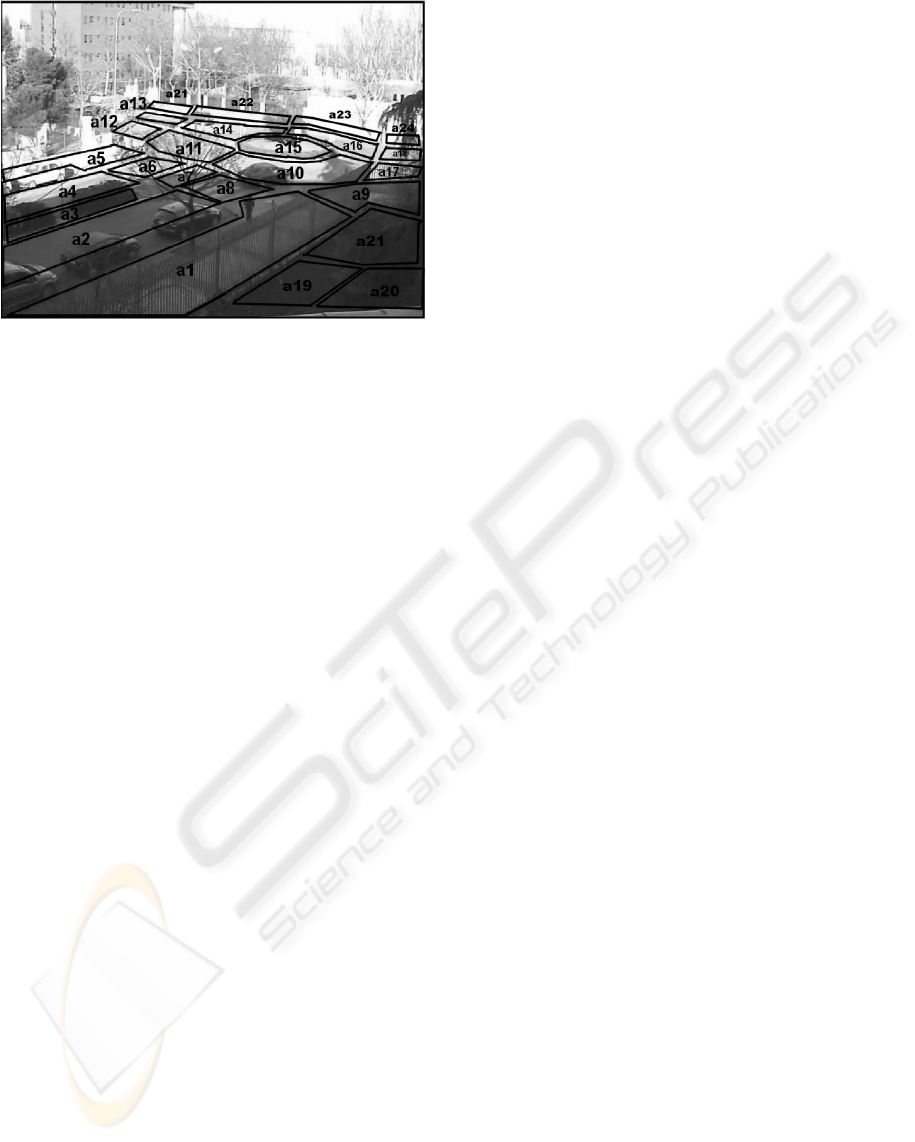
Figure 1: Capture of the studied environment and definition
of zones to represent the trajectories.
the possible zones where an object is located. The
knowledge base is completed with the definition of
normal trajectories. Figure 1 shows the studied scene
and the defined zones or areas. In the next section, we
introduce and formally define the trajectory concept.
3.2 Trajectory Definition
A trajectory is defined as a sequence of zones. In this
sequence, first and last zones represent the origin and
end of the trajectory, respectively. The trajectory def-
inition can be amplified with the association of con-
straints. A trajectory is correctly followed by one ob-
ject if the associated constrains are satisfied.
Formally, a trajectory t is defined from three ele-
ments:
t =< V;DDV;Φ > (1)
being V the set of input variables needed to de-
fine the trajectory t. Besides, DDV is the set of
domain definitions of each variable belonging to V.
Therefore, if V = {v
1
,v
2
,...,v
n
}, DDV is defined as
DDV = {DDV
1
,DDV
2
,...,DDV
n
}, where DDV
i
is the
domain definition of variable v
i
. Finally, Φ is the
set of constraints or conditions which can be used to
complete the trajectory definition according to the el-
ements of V (Φ = {µ
1
,µ
2
,...,µ
k
}).
In order to complete the definition of a trajec-
tory, three types of constraints are proposed: Role
constraint (who), specifies what types of objects are
allowed to follow the trajectory; Spatial constraint
(where), this type of constraints checks if objects cor-
rectly follow the sequence of defined areas and move
towards the destination; Temporal constraint (when),
allows to specify when moving objects can follow tra-
jectories.
Formally, a constraint is defined as a fuzzy set de-
fined over the domain P (V), with an associated mem-
bership function (µ
x
):
µ
x
: P (V) −→ [0, 1] (2)
This function returns a value within the inter-
val [0,1], where 1 represents the maximum satisfac-
tion degree of the constraint, and 0 represents the
minimum. Actually, constrains are fuzzy constraints
whose satisfaction degree is given by a membership
function µ
x
. Besides, the constraints represent a set
of conditions which must be satisfied by an object to
consider its behavior as normal.
The role constraint specifies what kind of objects
are allowed to follow a specific normal path. This
constraint is defined as a fuzzy set with the following
membership function:
µ
1
(obj) =

µ
c
(obj) if c ∈ ϒ;
0 in other case;
where µ
c
(obj) is the vague information about
what kind of object is obj. This information is ob-
tained from the lowest layer, where the video stream
is processed and objects are tracked. There is a mem-
bership function value for each class c. Finally, ϒ rep-
resents the set of classes/roles that are allowed to fol-
low the current trajectory.
On the other hand, we define two types of spatial
constraints: sequence and destination constraints. A
spatial sequence constraint associated to a trajectory
analyzes whether an object is following the sequence
of areas in order. To do that, the system updates the
list of possible areas in which an object is located
(ℓ(obj)) in each time. The function µ
2.1
associated
to this type of constraint is defined as follows:
µ
2.1
(obj) =



max(µ
a
(obj)) if ∃(µ
a
(obj) ∈ ℓ(obj))
| a ∈ Ψ ∧ a
prev
≤ a;
0 in other case;
where µ
a
(obj) is vague information in the low-
level layer about the object location. In other words,
µ
a
(obj) is a membership function value for fuzzy lo-
cations (∀a ∈ DDV
A
→ µ
a
(obj), being a one specific
area and A is the set of areas in the environment). On
the other hand, a
prev
is the previous area covered by
the object ob j. Initially, the value of the variable is the
beginning area or zone of the trajectory. Ψ denotes the
allowed sequence of zones, and max(µ
a
(obj)) is the
maximum value µ
a
(obj) ∈ ℓ(obj)|a ∈ Ψ. The symbol
≤ denotes an order relation in the sequence of areas
Ψ associated to one normal path, such that if a
′
≤ a
then, a
′
is the same area that a, or a is the next area
from a
′
in the sequence Ψ.
Destination constraints are used to determine if a
certain object is continuously getting closer to the end
area defined for a trajectory. In affirmative case, the
ICEIS 2009 - International Conference on Enterprise Information Systems
104

function returns 1. Otherwise, the value decreases un-
til 0 as the object goes away from the end area. In
other words, an object is less possible to follow the
trajectory as it goes away to the end area. The mem-
bership function µ
2.2
associated with this type of con-
straint is defined as follows:
µ
2.2
(d
i
,d
c
) =



1 if d
c
≤ d
i
1−
d
c
2∗d
i
if d
i
< d
c
< 2∗ d
i
0 if d
c
≥ 2∗ d
i
;
where d
i
and d
c
denote the initial and current dis-
tance between the object and the end area a
e
, respec-
tively. Initial distance refers to the distance between
the object and the end zone when it started to follow
the trajectory.
Finally, temporal constraints allow us to specify
when trajectories can be followed by moving objects.
Two types of temporal constraints are distinguished.
The first of them indicates the maximum duration al-
lowed for a trajectory and its membership function is
defined as follows:
µ
3.1
(t
max
,t
c
,t
b
) =

1 if t
max
= Ø∨t
max
≤ (t
c
− t
b
)
0 in other case;
Being t
c
the current time, t
b
the time in which
the object started to follow the trajectory, and t
max
the maximum duration allowed for the trajectory. An
object starts to follow a trajectory when it is situated
over the origin zone defined for that trajectory.
The second type of temporal constraint determines
the time interval that a trajectory must meet. Tempo-
ral constraints and relationships of simple events are
critical for representing and understanding composed
events. We define five temporal relationships which
are based on Allen’s interval algebra (Allen and Fer-
guson, 1994) and Lin’s work (Lin et al., 2008), as
shown in Table 1. These relationships are used to
check whether a normal path is being followed in a
particular interval.
The membership function µ
3.2
is built based on the
relationships given in Table 1:
Table 1: Temporal relationships between time instants and
intervals.
Temporal Relation Logical definition
Before t
c
< start(Int
j
)
After end(Int
j
) < t
c
During start(Int
j
) < t
c
< end(Int
j
)
Starts start(Int
j
) = t
c
Finish end(Int
j
) = t
c
µ
3.2
(Int
j
,t
c
) =





1 if (Int
j
= Ø) ∨Starts(t
c
,Int
j
)
∨ During(t
c
,Int
j
)
∨Finish(t
c
,Int
j
))
0 in other case;
An object satisfies a temporal restriction with an
associated time interval Int
j
if the current time t
c
be-
longs to the defined interval.
3.3 Detection of Anomalous Behaviors
The normality component described in this section
determines that an object is properly behaving if it is
following one or more normal trajectories. The belief
linked to an object obj that follows a concrete trajec-
tory t is calculated as follows:
b
t
(obj) =
|Φ|
^
x=1
µ
x
(3)
being
V
a t-norm, for example the t-norm mini-
mum. A high value of b
t
means that the object obj
is properly following the trajectory t, and a low value
represents the opposite case.
On the other hand, the normality of an object
obj according to the trajectory concept, denoted as
N(obj), is calculated as follows:
N(obj) =
w
_
y=1
b
t
y
(obj) (4)
where w is the number of trajectories and
W
is a
t-conorm, for example the t-conorm maximum. Actu-
ally, the normality analysis of an object obj is defined
as the result of a two-level fuzzy AND-OR network
applied to a set of constraints (by using the t-norm
minimum and the t-conorm maximum).
Finally, an object obj has a normal behavior ac-
cording to the trajectory concept when:
N(obj) > α (5)
being α a threshold defined by a security expert, who
takes advantage of previous experience to establish an
adequate value for this parameter. Normally, it takes
values from 0.2 < α < 0.5. Larger values of α in-
volve a stricter surveillance as the constraint satisfac-
tion value has to be larger to meet normality.
4 CASE STUDY: URBAN
ENVIRONMENT
In this section, we explain how the normality compo-
nent described in this paper works in a real environ-
INTELLIGENT SURVEILLANCE FOR TRAJECTORY ANALYSIS - Detecting Anomalous Situations in Monitored
Environments
105

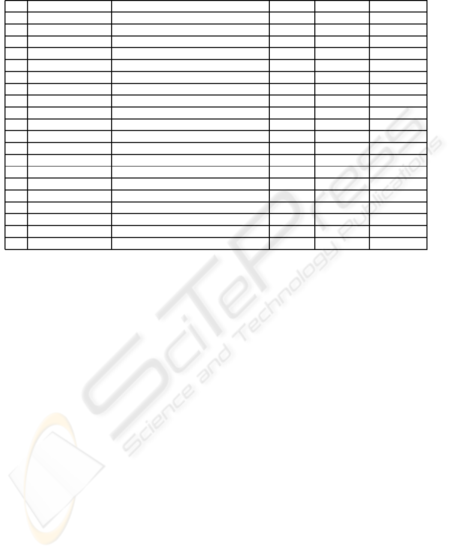
Table 2: Set of normal trajectories defined for the environment shown in Figure 1.
t µ
1
µ
2.1
µ
2.2
µ
3.1
µ
3.2
t
1
ϒ = {vehicle} Ψ = {a
2
,a
8
,a
10
,a
16
,a
14
,a
13
} a
e
= a
13
t
max
= 150 Ø
t
2
ϒ = {vehicle} Ψ = {a
2
,a
8
,a
10
,a
16
,a
14
,a
11
,a
6
,a
4
} a
e
= a
4
t
max
= 150 Ø
t
3
ϒ = {vehicle} Ψ = {a
2
,a
8
,a
10
,a
17
} a
e
= a
17
t
max
= 150 Ø
t
4
ϒ = {vehicle} Ψ = {a
18
,a
16
,a
14
,a
13
} a
e
= a
13
t
max
= 150 Ø
t
5
ϒ = {vehicle} Ψ = {a
18
,a
16
,a
14
,a
11
,a
10
,a
17
} a
e
= a
17
t
max
= 150 Ø
t
6
ϒ = {vehicle} Ψ = {a
18
,a
16
,a
14
,a
11
,a
6
,a
4
} a
e
= a
4
t
max
= 150 Ø
t
7
ϒ = {vehicle} Ψ = {a
12
,a
11
,a
6
,a
4
} a
e
= a
4
t
max
= 150 Ø
t
8
ϒ = {vehicle} Ψ = {a
12
,a
11
,a
10
,a
17
} a
e
= a
17
t
max
= 150 Ø
t
9
ϒ = {vehicle} Ψ = {a
12
,a
11
,a
10
,a
16
,a
14
,a
13
} a
e
= a
13
t
max
= 150 Ø
t
10
ϒ = {pedestrian} Ψ = {a
19
,a
20
} a
e
= a
20
Ø Int
j
= [US]
t
11
ϒ = {pedestrian} Ψ = {a
19
,a
21
,a
20
} a
e
= a
20
Ø Int
j
= [US]
t
12
ϒ = {pedestrian} Ψ = {a
20
,a
19
} a
e
= a
19
Ø Int
j
= [US]
t
13
ϒ = {pedestrian} Ψ = {a
20
,a
21
,a
19
} a
e
= a
19
Ø Int
j
= [US]
t
14
ϒ = {pedestrian} Ψ = {a
1
,a
9
} a
e
= a
9
Ø Ø
t
15
ϒ = {pedestrian} Ψ = {a
1
,a
8
,a
7
,a
6
,a
5
} a
e
= a
5
Ø Ø
t
16
ϒ = {pedestrian} Ψ = {a
5
,a
6
,a
7
,a
8
,a
1
} a
e
= a
1
Ø Ø
t
17
ϒ = {pedestrian} Ψ = {a
7
,a
8
,a
1
} a
e
= a
1
Ø Ø
t
18
ϒ = {pedestrian} Ψ = {a
7
,a
6
,a
5
} a
e
= a
5
Ø Ø
t
19
ϒ = {pedestrian} Ψ = {a
21
,a
22
,a
a23
,a
24
} a
e
= a
24
Ø Ø
t
20
ϒ = {pedestrian} Ψ = {a
24
,a
23
,a
22
,a
21
} a
e
= a
21
Ø Ø
ment. To do that, we have chosen a typical urban en-
vironment captured by a camera placed on our univer-
sity (see Figure 1). Once the areas have been defined
by an expert, the KB is completed with the definition
of the normal trajectories. Table 2 summarizes the set
of normal trajectories for the environment shown in
Figure 1.
In Table 2, every t
i
specifies a normal trajectory
which is followed when the constraints are satisfied.
[US] (University Schedule) is a time interval in which
the University is open for students. Some vehicle
paths have a temporal constraint with a maximum
time of 150 seconds. Higher times may mean traffic
jams or possible accidents.
Once the zones and normal trajectories have been
defined, the system uses the KB for analyzing where
an object could be located and the possible trajecto-
ries followed by it. Table 3 summarizes the normality
analysis results obtained after studying the trajecto-
ries followed by one car. Note that only four frames
have been included due to space limitations.
As can be appreciated in Table 3, the car has al-
ways associated a trajectory with a belief larger than
the value α. In other words, the normality value
N(obj) for the tracked car is always larger than the
threshold. Therefore, in this case, the object has a
normal behavior in each key instant.
5 CONCLUSIONS
In this paper we have proposed a system based prin-
cipally on the analysis of normality in order to detect
anomalous behaviors in real monitored environments.
This system is composed of normality components
which allow us to model the environment normality
and to specify how a certain object must ideally be-
have. Moreover, a normality component which ana-
lyzes the trajectories followed by an object has been
described in detail.
In the very near future, we will design new nor-
mality components in which machine learning algo-
rithms or knowledge acquisition tools will be used to
help the security expert to build the knowledge base
needed for behavior understanding. We will also pay
special attention to the information fusion from data
provided by different sensors to avoid wrong alarms.
This approach may help us to overcome the problem
of constraints non-fulfilment when information about
objects is incomplete or lost.
ACKNOWLEDGEMENTS
This work has been founded by the Spanish Ministry
of Industry (MITYC) under Research Project HES-
PERIA (CENIT Project).
ICEIS 2009 - International Conference on Enterprise Information Systems
106

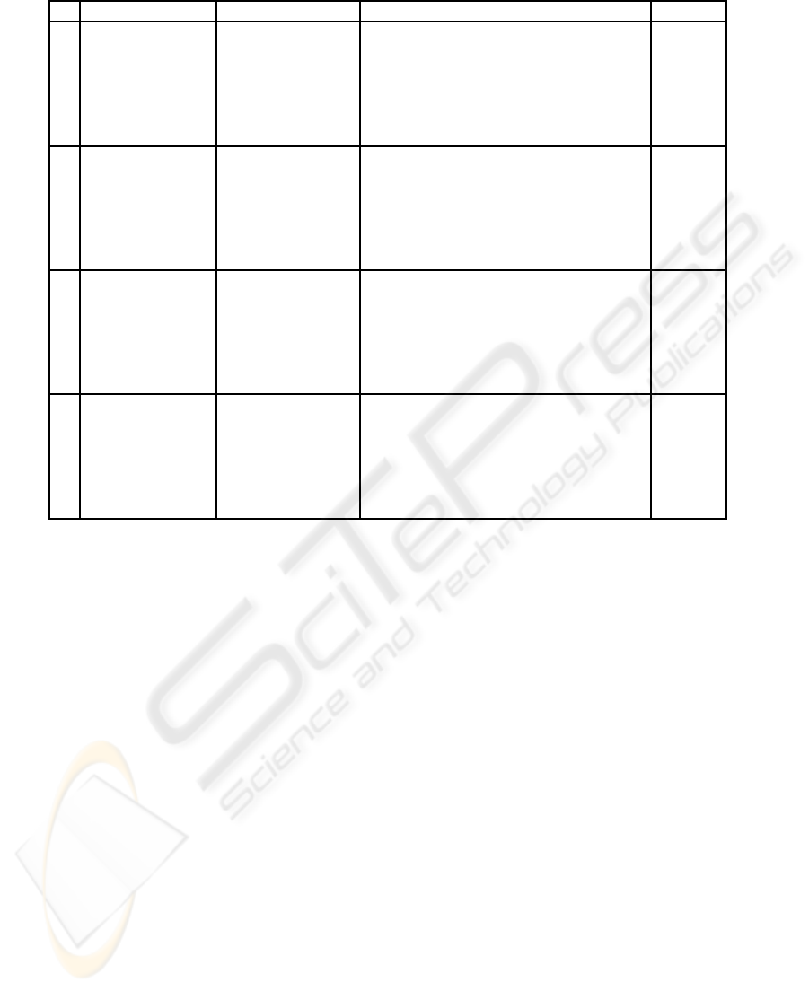
Table 3: Numeric values of normality analysis with α = 0.4.
t Classification Location Constraint values b
t
(obj)
1 µ
c
1
(obj1) = 1
µ
a
2
(obj1) = 0.8
t
1
→ {µ
1
= 1,µ
2.1
= 0.8, µ
2.2
= 1, 0.8
µ
a
3
(obj1) = 0.2
µ
3.1
= 1,µ
3.2
= 1}
t
2
→ {µ
1
= 1,µ
2.1
= 0.8, µ
2.2
= 1, 0.8
µ
3.1
= 1,µ
3.2
= 1}
t
3
→ {µ
1
= 1,µ
2.1
= 0.8, µ
2.2
= 1, 0.8
µ
3.1
= 1,µ
3.2
= 1}
3 µ
c
1
(obj1) = 0.9
µ
a
8
(obj1) = 0.4
t
1
→ {µ
1
= 0.9, µ
2.1
= 0.6, µ
2.2
= 1, 0.6
µ
c
2
(obj1) = 0.1
µ
a
10
(obj1) = 0.6
µ
3.1
= 1,µ
3.2
= 1}
t
2
→ {µ
1
= 0.9, µ
2.1
= 0.6, µ
2.2
= 1, 0.6
µ
3.1
= 1,µ
3.2
= 1}
t
3
→ {µ
1
= 0.9, µ
2.1
= 0.6, µ
2.2
= 1, 0.6
µ
3.1
= 1,µ
3.2
= 1}
5 µ
c
1
(obj1) = 0.7
µ
a
14
(obj1) = 0.7
t
1
→ {µ
1
= 0.7, µ
2.1
= 0.7, µ
2.2
= 1, 0.7
µ
c
2
(obj1) = 0.3
µ
a
22
(obj1) = 0.3
µ
3.1
= 1,µ
3.2
= 1}
t
2
→ {µ
1
= 0.7, µ
2.1
= 0.7, µ
2.2
= 0.6, 0.6
µ
3.1
= 1,µ
3.2
= 1}
t
3
→ {µ
1
= 0.7, µ
2.1
= 0.0, µ
2.2
= 0.3, 0.0
µ
3.1
= 1,µ
3.2
= 1}
6 µ
c
1
(obj1) = 0.7
µ
a
14
(obj1) = 0.3
t
1
→ {µ
1
= 0.7, µ
2.1
= 0.7, µ
2.2
= 1, 0.7
µ
c
2
(obj1) = 0.3
µ
a
13
(obj1) = 0.7
µ
3.1
= 1,µ
3.2
= 1}
t
2
→ {µ
1
= 0.7, µ
2.1
= 0.3, µ
2.2
= 0.5, 0.3
µ
3.1
= 1,µ
3.2
= 1}
t
3
→ {µ
1
= 0.7, µ
2.1
= 0.0, µ
2.2
= 0.1, 0.0
µ
3.1
= 1,µ
3.2
= 1}
REFERENCES
Allen, J. and Ferguson, G. (1994). Actions and events in
interval temporal logic. In Journal of Logic and Com-
putation, volume 4(5), pages 531–579.
Bauckhage, C., Hanheide, M., Wrede, S., and Sagerer, G.
(2004). A cognitive vision system for action recogni-
tion in office environments. In Computer Vision and
Pattern Recognition, Proceedings of the 2004 IEEE
Computer Society Conference on.
Collins, R., Lipton, A., Kanade, T., Fujiyoshi, H., Dug-
gins, D., Tsin, Y., Tolliver, D., Enomoto, N., and
Hasegawa, O. (2000). A system for video surveillance
and monitoring. In Technical report CMU-RI-TR-00-
12. Robotics Institute, Carnegie Mellon University.
Dee, H. and Hogg, D. (2004). Detecting inexplicable be-
haviour. In British Machine Vision Conference, pages
477–486.
Haritaoglu, I., Harwood, D., and Davis, L. (2000). w
4
:
Real-time surveillance of people and their activities.
In Patter Analysis and Machine Intelligence, volume
22(8), pages 809–830.
Henning, M. (2004). A new approach to object-oriented
middleware. In IEEE Internet Computing, volume
8(1), pages 66–75.
Hudelot, C. and Thonnat, M. (2003). A cognitive vision
platform for automatic recognition of natural complex
objects. In International Conference on Tools with Ar-
tificial Intelligence, ICTAI, pages 398–405.
Johnson, N. and Hogg (1996). Learning the distribution
of object trajectories for event recognitio. In Image
and Vision Computing, Elsevier, volume 14(8), pages
609–615.
Lin, L., Gong, H., Li, L., and Wang, L. (2008). Semantic
event representation and recognition using syntactic
attribute graph grammar. In Pattern Recognition Let-
ters, ARTICLE IN PRESS.
Makris, D. and Ellis, T. (2002). Path detection in video
surveillance. In Image and Vision Computing, volume
12(20), pages 895–903.
Piciarelli, C., Foresti, G., and Snidaro, L. (2005). Trayec-
tory clustering and its applications for video surveil-
lance. In IEEE Conference on Advanced Video and
Signal Based Surveillance, pages 40–45.
Wang, W. and Maybank, S. (2004). A survey on visual
surveillance of object motion and behaviors. In Sys-
tems, Man and Cybernetics, Part C, IEEE Transac-
tions on, volume 34(3), pages 334–352.
Zadeh, L. (1996). Fuzzy sets. Fuzzy Sets, Fuzzy Logic, and
Fuzzy Systems: Selected Papers.
INTELLIGENT SURVEILLANCE FOR TRAJECTORY ANALYSIS - Detecting Anomalous Situations in Monitored
Environments
107