
Disparity Measure Construction for Comparison of
3D Objects’ Surfaces
Natalya Dyshkant
Department of Computational Mathematics and Cybernetics
Lomonosov Moscow State University
Vorobyevy gory, Moscow, Russian Federation
Abstract. In this paper a problem of 3D objects’ surfaces comparison is consid-
ered. Each spatial object is given as a set of schlicht surfaces that are described
by point clouds. This article discusses a proposed disparity measure to compare
such objects and an algorithm to compute it. A method for comparison of mesh
functions defined on different point sets is proposed. The theoretical base of the
proposed approach is the piecewise-linear approximation of surfaces using De-
launay triangulations for initial point clouds. The presented approach uses Delau-
nay triangulations of each point clouds, general Delaunay triangulation for both
clouds, function interpolation on basis of localization of triangulations in each
other and function comparison on single cells of general triangulation. Local-
ization is implemented on basis of minimum spanning trees. As the application
of the proposed methodology a problem of 3D face models comparison is con-
sidered. It was experimentally verified that the proposed method is numerically
efficient.
1 Introduction
In pattern recognition, along with k-nearest neighbors, estimate evaluation ([1]) and
other algorithms there is a method of pattern matching. A problem of metrics construc-
tion for comparison of a given object with the standard occurs in biometric identification
(e.g. by 3D face model) and various medical applications.
Any spatial object has a certain geometric shape. Objects’ shape can be considered
as a set of schlicht surfaces. In such a way a problem of object comparison reduces to a
problem of surface comparison.
A method of pointwise description is usually used for specification of complex
uneven surfaces. Then a surface is considered as a discrete nonregular ensemble of
points. One can receive such description using 3D scanning methods (e.g. http://artec-
group.com), topographic mapping and some other.
As the result of rapid progress in objects’ 3D scanning techniques problems con-
nected with received surfaces analysis and comparison occur.
Accurate and numerically efficient algorithms of computing disparity measure be-
tween surfaces are required in many applications of computer graphics. It is necessary
to compare surfaces solving problems of surface classification, surface reconstruction
by its separate fragments, etc.
Dyshkant N. (2009).
Disparity Measure Construction for Comparison of 3D Objects’ Surfaces.
In Proceedings of the 2nd International Workshop on Image Mining Theory and Applications, pages 43-52
DOI: 10.5220/0001957300430052
Copyright
c
SciTePress

Known approaches to compare piecewise linear functions that are defined on differ-
ent discrete sets use hash functions [2]. They have quadratic computational complexity
at worst and so are too computationally intensive.
Our method based on constructing of general Delaunay triangulations for union of
two discrete sets. As the merging process can be implemented in linear time ([8]) then
the total time to compute the proposed measure is comparable with time to construct
Delaunay triangulation, i.e. O(N log N ), where N — the total amount of points in two
sets. Consequently, the proposed method allows to avoid quadratic search in surface
comparison that determines its advantage and novelty.
This paper is organized as follows. In section 2, we describe problem definition
and introduce the proposed disparity measure. In section 3, each of stages of the pro-
posed algorithm for disparity measure calculation is described. In section 4 we discuss
application of the proposed method for 3D face model comparison. The results of com-
putational experiments are given in section 5.
2 Problem Definition and Basic Ideas
A finite point set G : {(x
i
, y
i
) ∈ R
2
|i = 1, . . . , N }, N ≥ 3 is called a nonregular
two-dimensional mesh.
We consider the following problem definition.
Let G
1
= {(x
i
1
, y
i
1
)}
N
1
i=1
and G
2
= {(x
2
1
, y
2
1
)}
N
2
i=1
be nonregular 2D meshes. Sup-
pose F
1
and F
2
are the mesh functions corresponded to G
1
and G
2
, i.e.
F
1
= {f
i
1
}
i=1
N
1
, f
i
1
= F
1
(x
i
1
, y
i
1
); F
2
= {f
i
2
}
i=1
N
2
, f
i
2
= F
2
(x
i
2
, y
i
2
).
It is required to introduce a metrics for comparison such mesh functions and to
design a numerically efficient algorithm to compute it.
Let R be a rectangle in R
2
. Let µ(x, y) be a function that defines weight of frag-
ments of R in accordance with significance of function similarity on each fragment.
By G denote the set of nonregular 2D meshes contained in R. Consider a set F of
single-valued functions on meshes from G.
Now we introduce a proximity function ρ over set F.
By Conv(G) denote the convex hull of G. Consider F
1
, F
2
∈ F. Let
ˆ
F
1
and
ˆ
F
2
be
continuous functions defined on Conv(G
1
) ∩Conv(G
2
) such that
ˆ
F
1
≡ F
1
on G
1
and
ˆ
F
2
≡ F
2
on G
2
. By T denote the Delaunay triangulation of mesh G
1
∪ G
2
. We will
say that this mesh is the general mesh and T is the general Delaunay triangulation. Let
A, B, C be points of the general mesh. By definition, put
V (A, B, C, F
1
, F
2
) =
ZZ
△ABC
ˆ
F
1
(x, y) −
ˆ
F
2
(x, y)
µ(x, y) dxdy. (1)
The value of V indicates a weighted volume between two surfaces defined by func-
tions F
1
and F
2
over triangle △ABC.
We are interested in case when Conv(G
1
)∩Conv(G
2
) 6= ∅. Otherwise two objects
should be reduced to such coordinate system that allows them to be comparable.
44

Then we introduce a proximity function ρ as
ρ(F
1
, F
2
) =
X
△ABC∈T
V (A, B, C, F
1
, F
2
). (2)
So we compute disparity measure for two surfaces summing values of volume be-
tween them over all triangles △ABC of general triangulation T .
We introduce disparity measure between two surfaces as a spacial volume between
the corresponding functions. It is also allowed to use ”weighted” volume. In this case
similarity of some surface patches will have weight greater than similarity of others.
Let us remark that two functions F
1
and F
2
are defined on different meshes. The
basic idea of the proposed approach is to fill values of each functions at points of the
other mesh using construction of two triangulations and their localization in each other.
3 Methods
The following stages will be performed to compute the disparity measure 2 between
two surfaces given by functions F
1
and F
2
.
1. Delaunay triangulation for each of the meshes G
1
, G
2
is constructed;
2. each of two meshes G
1
, G
2
is located in the triangulation for the other mesh;
3. each of two functions F
1
, F
2
is interpolated on the mesh that the other function is
defined on;
4. the general triangulation of both meshes G
1
∪G
2
is constructed on basis of unsep-
arated triangulation merging;
5. after that in each point of the general mesh values of two functions are known, and it
is possible to make comparison operation on particular cells of the general triangu-
lation, analyzing positional relationship of the spatial triangles given by functions.
Let’s consider each of steps in detail.
3.1 Delaunay Triangulation Construction
A triangulation T for a set G is called Delaunay triangulation if the following condition
holds: there is no point in G is inside the circumcircle of any triangle in T (see Figure).
The used triangulation construction algorithm based on the paradigm of recursive
decomposition (”divide-and-conquer strategy”): division of initial set into two approxi-
mately equal subsets, recursive triangulation construction of these subsets and merging
of two divided triangulations. The data structure ”nodes with neighbors”, described in
[3], can be used.
Computational complexity of this algorithm is O(N log N).
45
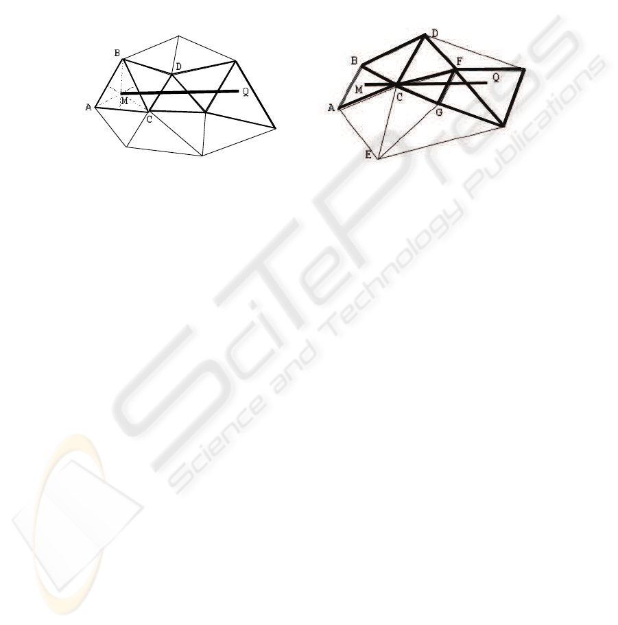
3.2 Point Location in Triangulation
To locate point Q in a Delaunay triangulation T means to declare the triangle of T
containing this point. In cases of (i) coincidence of point Q and one of triangulation
vertices; (ii) belonging of point Q to one of triangulation edges, it is possible to declare
any of triangles incident to the specified vertex or to the specified edge. In case of point
Q oversteps the boundaries of T it is possible to declare certain infinite triangle or the
nearest triangle to this point.
Fig.1. Point location in triangulation. Fig.2. Point C of triangulation belongs to seg-
ment [MQ].
Let point M be a point that location in the triangulation is known (e.g. it can be
the center of the inscribed circle of any triangle). The idea of algorithm solving point
location in triangulation problem consists in gradual transition from M to Q along the
straight line (M Q). During each transition step changing on adjacent (neighboring by
side) triangle is implemented. Case of belonging of a certain point of T to segment
[MQ] is a case of a special interest (see Figure 2). A similar algorithm was described
in [4].
Thus, after point location stage is finished, there is a path consisting of triangulation
triangles, each of them (except the initial one) is adjacent with previous. We say that it
is location path. On Figures 1 and 2 triangles of location path are outlined.
Complexity of one point location depends on quantity of triangles located along
segment [MQ] and is O(
√
N) on the average and O(N) at worst.
3.3 Mesh Location in Triangulation
To locate a two-dimensional mesh G in a triangulation T means to locate all points of
G in this triangulation.
We propose a mesh location algorithm that uses spanning tree for graph T . In this
case location paths will pass along edges of spanning tree.
As spanning tree for graph T does not contain cycles and passes through all points
of the mesh G, the algorithm will work correctly: it will not loop and performs location
of absolutely all points of mesh.
The proposed method for comparison of schlicht surfaces uses the general triangu-
lation of two meshes constructed by merger method on one of the subsequent stages.
46
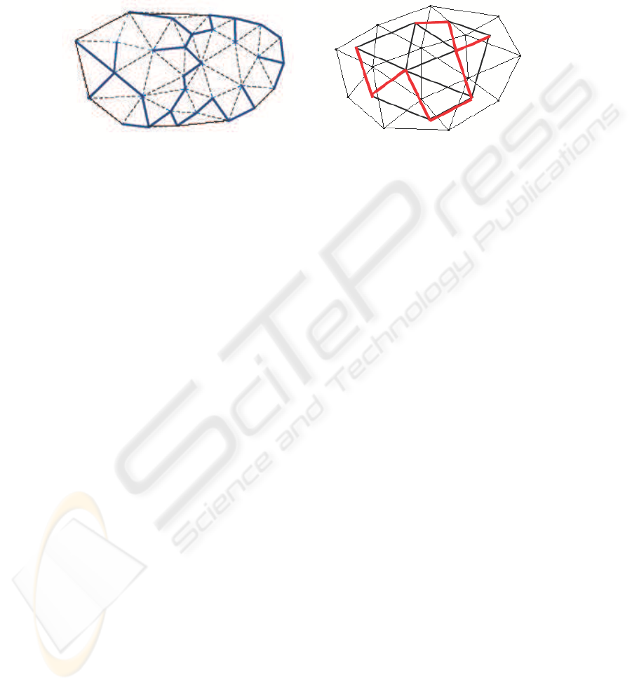
This method uses minimum spanning trees (MST) of both meshes. So it is justified
to use exactly minimum spanning trees for mesh location. Then location paths will be
optimal (see Fig. 3, 4).
Fig.3. Minimum spanning tree for Delaunay
graph.
Fig.4. Mesh location in triangulation.
It is known, that it is possible to construct minimum spanning tree for a set G from
Delaunay triangulation for G in linear time. Linear time is reached owing to clean-
up operation proposed by Cheriton and Tarjan in [5], and to data structure ”fibonacci
heap”, defined by Fredman and Tarjan in [6], [7].
It was experimentally verified that computational complexity of mesh location stage
is O(N ).
By means of the described algorithm each of the meshes G
1
and G
2
is located in the
triangulation for the other mesh, and it is possible to consider a problem of interpolation
for function given on one mesh at points of the other mesh.
3.4 Function Interpolation
Let point V
0
(x
0
, y
0
) be located in a certain triangle △(V
1
(x
1
, y
1
), V
2
(x
2
, y
2
), V
3
(x
3
, y
3
)):
such that F (x
1
, y
1
) = f
1
, F (x
2
, y
2
) = f
2
, F (x
3
, y
3
) = f
3
. For interpolation of func-
tion F value at the point V
0
linear interpolation and barycentric coordinates can used:
f
0
= λ
1
f
1
+ λ
2
f
2
+ λ
3
f
3
, here λ
1
λ
2
λ
3
≥ 0 and
x
0
= λ
1
x
1
+ λ
2
x
2
+ λ
3
x
3
;
y
0
= λ
1
y
1
+ λ
2
y
2
+ λ
3
y
3
;
1 = λ
1
+ λ
2
+ λ
3
.
Results of the described method are shown on Figures 5 - 8. The triangulated surface
defined by function F
1
on grid G
1
is represented by (1) (on the top), the triangulated
surface defined by function F
2
on grid G
2
is represented by (2) (at the bottom of Figure
5) and the surface received after interpolation of function F
2
on grid G
1
is represented
by (3) (at the bottom). As shown on Figures, two triangulations represented by (2) and
(3) define the same surface (the bottom one).
Computational complexity of mesh interpolation stage is O(N ).
47
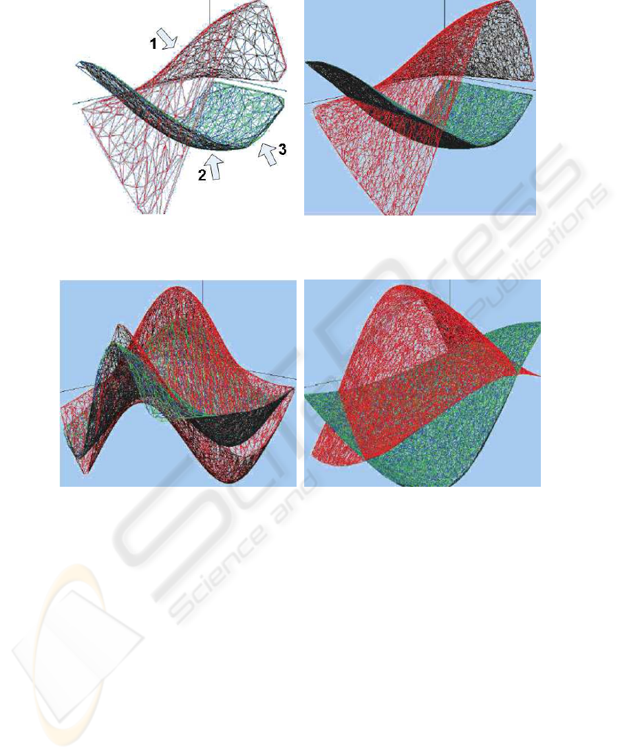
Fig.5. Linear interpolation, N
1
= N
2
=
1 000.
Fig.6. Linear interpolation, N
1
= N
2
=
10 000.
Fig.7. Linear interpolation, N
1
= N
2
=
10 000.
Fig.8. Linear interpolation, N
1
= N
2
=
15 000.
By means of the described method values of function F
1
are interpolated at all
points of mesh G
2
and values of function F
2
are interpolated at points of mesh G
1
.
3.5 Function Comparison at Cells of General Triangulation
After interpolation stage values of two functions are known at each point of the general
mesh G = G
1
∪ G
2
: one of them has been given, and the second one is received by
interpolation.
Let’s construct the general Delaunay triangulation T for general mesh G. As loca-
tions for points of the meshes G
1
and G
2
in triangles of triangulationsfor G
2
and G
1
are
known usage of the triangulation merge algorithm proposed by L.Mestetkiy, E.Tsarik
in [8] is the most efficient here.
48
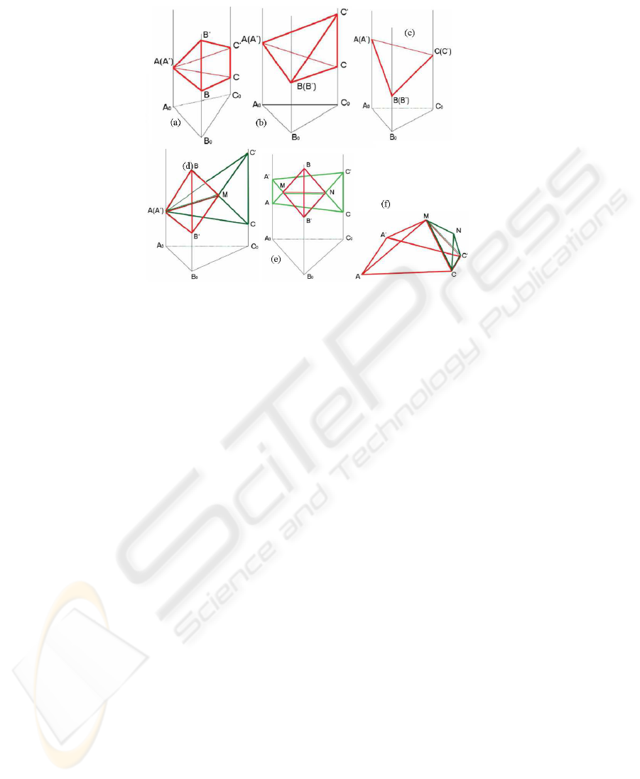
Fig.9. Comparison of functions given at three points: (a) a = 0, b > 0, c > 0; (b) a = 0, b = 0,
c > 0; (c) a = 0, b = 0, c > 0; (d) a = 0, b < 0, c > 0; (e) a > 0, b < 0, c > 0; (f) wedge
volume as sum of volumes of triangular or quadrangular pyramids.
Let △A
0
B
0
C
0
be a triangle of the general triangulation T and let △ABC and
△A
′
B
′
C
′
be spatial triangles corresponding to functions F
1
and F
2
. As a disparity
measure of surfaces we will use the sum of volumes of difference between prisms
A
0
B
0
C
0
ABC and A
0
B
0
C
0
A
′
B
′
C
′
over all triangles △A
0
B
0
C
0
of the general tri-
angulation T .
Let a, b, c be differences of coordinates of axis Oz of points A
′
and A, B
′
and B, C
′
and C respectively. We analyze positional relationships of the spatial triangles △ABC
and △A
′
B
′
C
′
and consider all possible cases (see Fig. 9). For computing of volume of
difference between prisms it is necessary to calculate volume of a pyramid — triangular
or quadrangular(see Fig. 9a-c), or total volume of two triangular pyramids (see Fig. 9d),
or total volume of a triangular pyramid and a wedge (see Fig. 9e) where wedge volume
is searched as the sum of volumes of quadrangular and triangular pyramids (see Fig.
9f).
Summing over all triangles of general triangulation value of difference volume, we
obtain the difference measure 2 between the given surfaces.
4 Comparison of Human Face Surfaces
As the application of the proposed methodology we have considered a problem of com-
parison of 3D face models (see Fig. 10).
Using elementary manipulations of one model (shifts and rotations by small angles)
it is possible to improvethe received result considerably,i.e. to find such model position
49
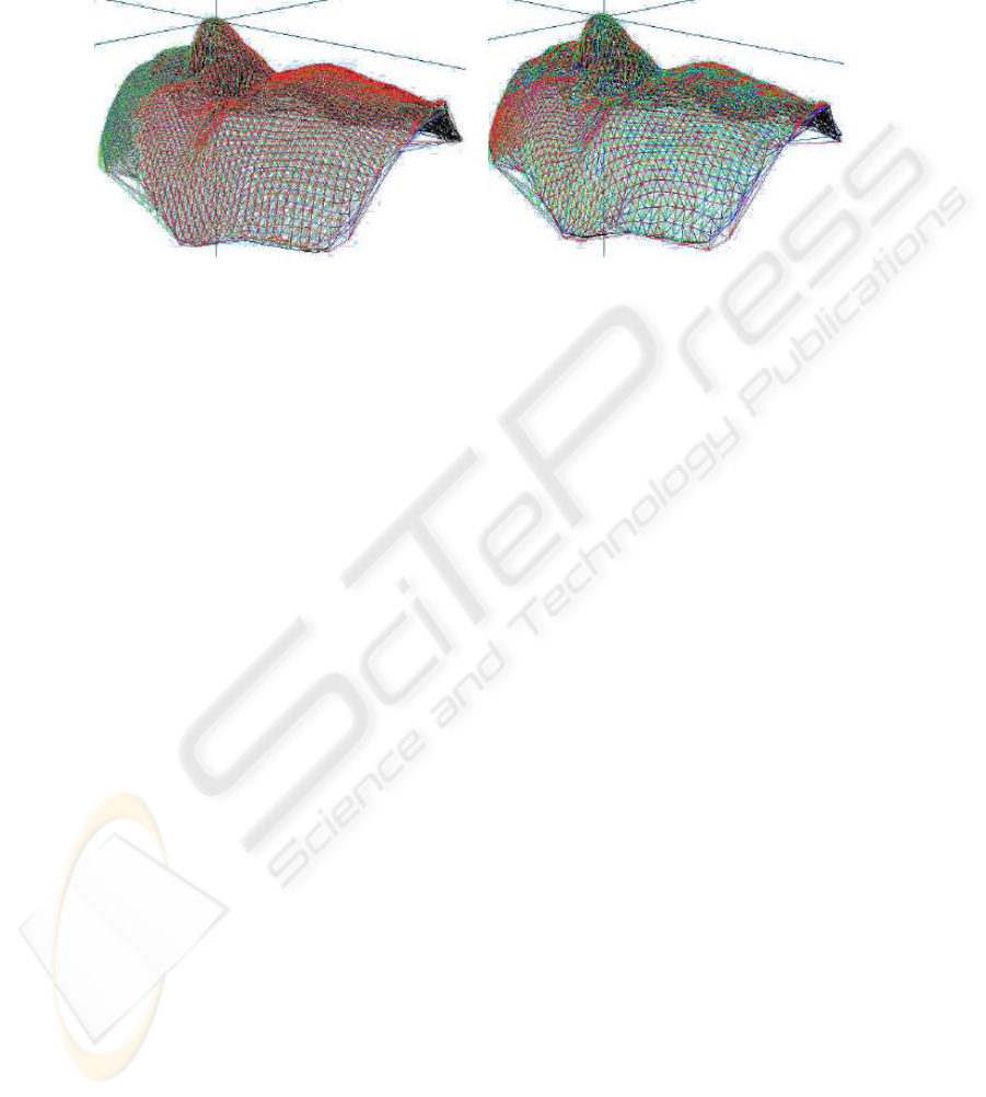
that two models constitute a maximum matching so that the corresponding disparity
measure will be minimal (see Fig. 11).
Fig.10. Comparison of 3D face models, dispar-
ity measure is 39 234, 254.
Fig.11. Comparison of 3D face models, dispar-
ity measure is 20 238, 8.
In [9] the author considered a problem of quantitative estimation of facial asymme-
try in 3D models. To solve this problem reflection of the initial model is constructed and
two models are compared using the presented approach. The received disparity measure
is called initial quantitative estimation of asymmetry. Then the correction stage of facial
asymmetry plane is performed and a final value of estimation is received.
5 Computing Experiments
The proposed method of surface comparison was implemented, and there also has been
made multiple computing experiments for all stages of algorithm.
As experimental estimations have shown, each of stages except stage of triangula-
tion constructions is implemented for linear time in number of mesh points. The stage
of triangulation construction is implemented for time O(N log N ), which defines com-
putational complexity of the proposed approach.
Running time for different stages of algorithm during surface comparison are ad-
duced in tables (1)-(3). The three-dimensional portraits consisting approximately from
3 000 points were used here. Computing experiments were carried out using AMD
Athlon 2 600+ processor and 512 Mb operative memory.
Let us remark that in case one of two models is stored in a database (verification
problem) then the total running time will cut in half because construction of Delaunay
triangulation and minimum spanning tree for stored model can be implemented during
preprocessing stage.
In addition, we have performed computing experiments on 3D face database that
estimate approximation accuracy of scanned surfaces. These experiments have showed
how much surfaces can be simplified without loss of accuracy for disparity measure (2)
by comparing initial triangular meshes and their simplified representation. The problem
50

Table 1. Running time for different stages of algorithm. Comparison of face surfaces consisting
of about 3 000 points.
Stage of algorithm Time (sec)
Construction of two triangulations 0,124
Construction of two MSTs 0,203
Location of triangulations 0,015
Function interpolation < 0,001
Construction of general triangulation 0,031
Computing disparity measure
R
F
1
− F
2
0,031
Total time 0,405
Table 2. Time for minimum spanning tree construction for graph of Delaunay triangulation using
Cheriton and Tarjan algorithm.
Number of points 20000 40 000 60000 80000 100 000
Time (sec) 0,906 1,812 2,562 3,531 4,468
Table 3. Time for location of one mesh in triangles of the triangulation for the other mesh.
Number of points in the mesh G
1
10000 25 000 50000 75 000 100 000
Time (sec) 0,031 0,093 0,171 0,234 0,312
Table 4. Running time of linear interpolation of both functions.
Number of points in both meshes G
1
and G
2
50000 100 000 150 000 200 000
Time (sec) 0,015 0,031 0,046 0,062
of measuring error on simplified surfaces were considered in detail by F.Cignoni et al
in [10].
6 Conclusions
A new approach to 3D objects’ surface comparison is proposed in this paper. A new
disparity measure between two surfaces is introduced. The approach is based on the
piecewise-linear approximation of surfaces using Delaunay triangulations for initial
point clouds.
The proposed method has the following advantages: numerical efficiency, possibil-
ity of paralleling. Besides, the described approach possesses some universality in com-
parison with others as it is suitable for comparison of any models given by functions on
discrete sets. The proposed measure can be adapted for each concrete application, for
example, by means of introducing measure on a surface. So the considered methodol-
ogy gives mathematical apparatus for construction of common and specific metrics for
surface comparison.
51

Acknowledgements
The author is grateful to her scientific adviser Prof. Leonid Mestetskiy for useful dis-
cussions and important observations. This work is supported by the Russian Foundation
for Basic Research (grants 08-01-00670, 08-07-00305-a).
References
1. Yu. I. Zhuravlev and V. V. Nikiforov, Recognition Algorithms Based on Estimate Evaluation,
Kibernetika, No. 3, 111 (1971).
2. Petrenko, D. A., S. A. Triangulation comparison using hash-functions (in russian). In Herald
of Tomsk State University 280 (2003).
3. Scvortsov, A. V. Delaunay triangulation and its applications (in Russian). Tomsk (2002).
4. Ernst, M., I. S. Fast randomized point location without preprocessing in two- and three-
dimensional delauney triangulation. In Proceedings of the 11th Annual Symposium on Com-
putational Geometry. Los Alamos, New Mexico (1996).
5. Cheriton, D., Tarjan, R. Finding minimum spanning trees. In SIAM J.Comput. (1976).
6. Fredman, M., Tarjan, R. Data Structures and Network Algorithms. Society for Industrial
and Applied Mathematics, London (1989), 2nd edition.
7. Tarjan, R. Fibonacci heaps and their uses in improved network optimization algorithms. In
Journal of the ACM (1987).
8. Mestetskiy, L., Tsarik, E. Delaunay triangulation: recursion without space division of ver-
tices (in russian). In GraphiCon, International Conference on computer graphics. Moscow
(2004).
9. Dyshkant, N., Mestetskiy, E. Asymmetry estimation in 3D faces (in russian). In Intellectual
Data Processing’08, pp.94-96, Simferopol (2008).
10. P. Cignoni, C. Rocchini and R. Scopigno Metro: measuring error on simplified surfaces.
Computer Graphics Forum, Blackwell Publishers, vol. 17(2), pp. 167-174, (1998).
52
