SIMULATION OF FOREST EVOLUTION
Effects of Environmental Factors to Trees Growth
Jing Fan
1
, Xiao-yong Sun
1,2
1
The Lab of Software Development Environment, Zhejiang University of Technology, Hangzhou 310014, China
2
School of Information and Electronic Engineering, Zhejiang University of Science and Technology
Hangzhou 310014, China
Ying Tang, Tian-yang Dong
The Lab of Software Development Environment, Zhejiang University of Technology, Hangzhou 310014, China
Keywords: Tree Growth Model, Forest Evolution Model, Forest Gap Model.
Abstract: Out of the complexity and variety of plant communities, it is a challenging task to simulate the structure and
dynamics of plant communities. In this paper we simulate and visualize the evolution of forests by the tree
growth model influenced by the environmental factors. The environmental factors we considered include
illumination, terrains and resource competition among trees. We develop our tree growth model based on
the forest gap model by effectively incorporating the above environmental factors. The system is
implemented with Visual C++ 6.0 and OpenGL. We compare the growth of trees (their heights and DBHs)
which are of different ages or located in different regions. We also show changes of trees distribution within
certain landscape for a long period of time (more than two hundred years). The illuminating and interesting
experimental results show that our simulation technique is effective.
1 INTRODUCTION
Realistic simulation of ecosystems is a challenging
topic, which involves bio-physics, ecology and
human aspects. We define the distributions of plants
across a plant community for a large period of time
as the space-time distribution model of the plant
community. This model determines the evolution of
the whole plant community. In our study, we focus
on the forest composed by several hundred trees. But
only one kind of tree is discussed in this paper. More
species of trees would be considered in the future
study. We need to consider the interactions of trees
with each other as well as the interactions with their
environment to determine the space-time distribution
model of the whole forest.
In this paper, we extend the method discussed by
Sang Weiguo and Li Jingwen (Sang and Li, 1998) to
develop our space-time distribution model. Our
model incorporates the terrain as the influence factor
which has not been considered in previous models.
Actually, we adopt a two-level model, where the
higher-level model determines the distribution of
trees (their numbers and locations) in macro scale,
and lower-level model determines the tree specific
parameters (heights and DBHs) in micro scale.
The structure of the paper is arranged as follows.
In the next section we briefly review previous
related work on this topic. Section 3 introduces
architecture of the system. In section 4 we describe
the detailed specific models and implementation
techniques. The simulation results are shown in
section 5. Section 6 gives the final conclusion.
2 PREVIOUS WORK
Modelling and visualization of ecosystem is a
difficult subject, mainly because of the complex
interactions at various time and space. To simulate
the distribution of plant community, University of
Calgary extended the L-system and introduced
Multiset L-system (Lane and Prusinkiewicz, 2002).
L-system can be used to model the individual plant
(Prusinkiewicz et al., 2001). An L-system model
66
Fan J., Sun X., Tang Y. and Dong T. (2009).
SIMULATION OF FOREST EVOLUTION - Effects of Environmental Factors to Trees Growth .
In Proceedings of the 11th International Conference on Enterprise Information Systems - Human-Computer Interaction, pages 66-71
DOI: 10.5220/0001990300660071
Copyright
c
 SciTePress

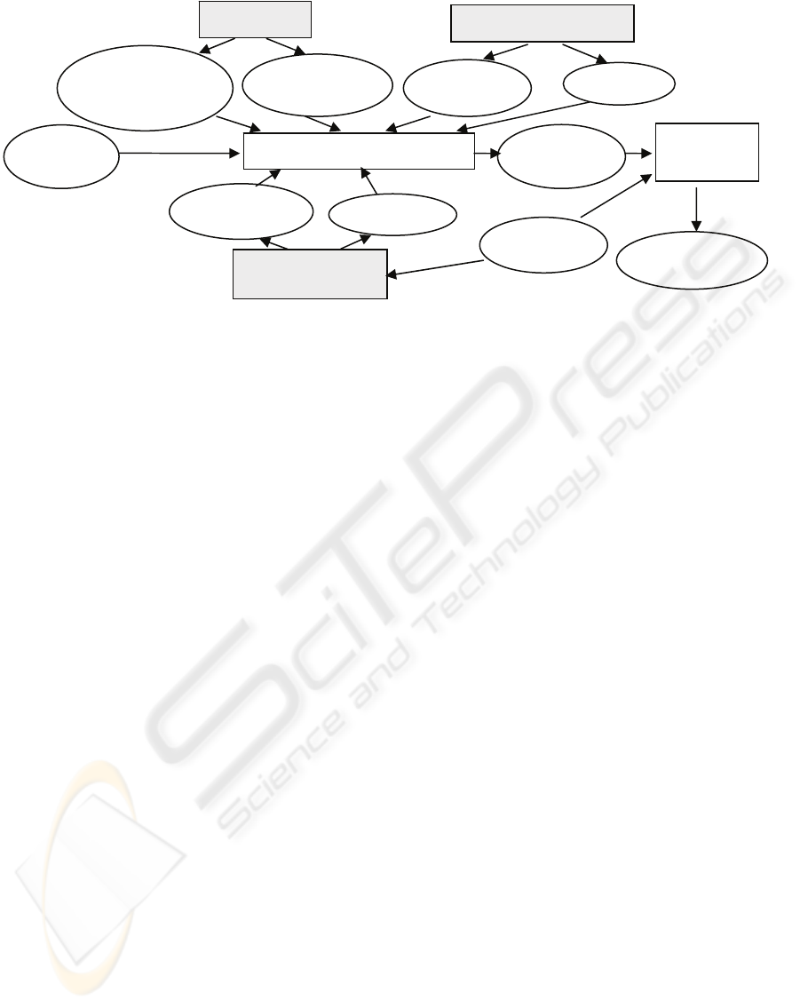
Figure 1: Forest evolving simulation system.
generates plants represented as strings of symbols
with optional parameters (Prusinkiewicz and
Lindenmayer, 1990). In Multiset L-system, the set of
productions operates on a multiset of strings that
represent many plants, rather than a single string that
represents an individual plant. New strings can be
dynamically added to or removed from this multiset,
representing organisms that are added to or removed
from the population. Based on Multiset L-system,
Lane et al. (Lane and Prusinkiewicz, 2002) proposed
a spatial distribution model of plants with the
ecologically and visually important phenomena of
clustering and succession of plants. The
shortcomings of this approach are mainly the lack of
retro-action between elements of the environment, as
well as unrealistic dynamics.
GreenLab model which is based on Source-Sink
Model and plant automation has been used in many
plant simulation applications. It is a
functional-structural model, which means that it
combines both functional growth and structure
development, interacting together (De Reffye and
Hu, 2003). But currently GreenLab model is mainly
applied to agriculture, and the research of
applications in forestry is still in the very early stage.
There are a lot of problems to be solved.
Forest gap model is one of the most active areas
in research of forest ecology. It is a forest evolving
model (Sang et al., 1999). In forest gap model
regeneration, mortality and growth of trees are
influenced by their neighbors. In our system the
forest gap model is extended with the terrain. We
implement the system with
Visual C++ 6.0 and
OpenGL, and the result is satisfying.
3 SYSTEM ARCHITECTURE
In order to make our system scalable, it is designed
to consist of three modules: tree growth module,
environment module and visualization module. And
the environment module includes temperature
model, light model and competition model. The
whole system architecture is shown in Figure 1.
3.1 Tree Growth Module
This module mainly includes the tree growth
equations. The basic idea is that we first establish
the tree growth function for the ideal state and later
modify it by considering environmental factors. The
values, which reflect the effects of different
environment factors on tree growth, are to be
computed in following environment module. Such
computed values are mapped into the ideal growth
function to get the actual growth of each tree. We
establish a tree growth influence function for each
kind of resource, the function will return a value in
[0, 1] based on the resource condition. If the value
equals 1, it means the resource is in its ideal state. If
the value equals 0, it means trees can not survive in
such environment. If the resource is inadequate or
too much, the value is a positive number less than 1,
then the tree growth will slow down.
In this module we only focus on the increase of
tree’s height and diameter at breast height (DBH),
the topological structure of tree will be ignored.
Such simplification speeds up the computation
greatly, yet it also provides enough information for
illuminating visualization.
DEM data
Light Model
Temperature model
Competition Model
Tree growth module
Initial data
of trees
Tree growth
data file
Visualization
Module
Scene rendered
Intensity at
different position
in canopy
Accumulative
leaf area index
Competition
facto
r
Biomass
Temperature
facto
r
Tree position
SIMULATION OF FOREST EVOLUTION - Effects of Environmental Factors to Trees Growth
67

3.2 Environment Module
Usually, the resource is not distributed uniformly
across the forest. As we all know, temperature
changes with height, slope direction will affect the
amount of light, so the resource distribution needs to
be modelled based on terrain.
In our system, the environment module includes
temperature model, light model and competition
model (Figure 1). As we have explained before, in
the tree growth module each environment factor is
represented by a value in [0, 1] which is computed in
the environment module. The process to compute
such coefficients is independent of the tree growth
model, which makes the environment module
scalable. If a new resource factor is introduced, the
tree growth module needs not to be modified. What
we need to do is just to add this resource to the
environment module to get the value that is to be
mapped into the tree grow function.
3.3 Visualization Module
Tree growth data including height and DBH are
computed in tree growth module. These growth data,
together with other tree information such as position,
age of trees and so on, are written into a binary file
as the input of visualization module. Visualization
module renders the terrain scene with digital
elevation map (DEM), and visualizes the trees’
distribution based on the input data.
4 SPACE-TIME DISTRIBUTION
MODEL OF FOREST AND ITS
IMPLEMENTATION
In our system we extend the forest gap model to
establish a space-time distribution model of forest
including the tree growth model and the
environment model.
4.1 Tree Growth Model
In this model growth, maturation and regeneration of
trees must be taken in account, so the sub models are
shown as follow.
4.1.1 Regeneration Model
If the regeneration takes place, number of
regeneration is determined by (Sang and Li, 1998):
!
)(P
n
e
n
n λ
λ
−
=
(1)
where
λ is the Poisson distribution parameter which
represent the average number of tree regeneration, n
is the number of tree regeneration, P(n) is the
probability of regeneration number being n.
4.1.2 Mortality Model
The change in number and distribution of trees in
forest is the result of regeneration and mortality
which are carrying on at the same time. The
mortality of the trees which grow normally is
computed by (Sang and Li, 1998):
n
M )1(1
0
ε −−=
(2)
where n is the age of a tree, M
0
is the mortality of a
tree at the age of n,
ε is the annual mortality rate.
4.1.3 Growth Model
The tree growth equation in ideal state is given
below (Sang and Li, 1998):
dzzzPS
dt
HDd
H
B
L
∫
−= ])([
)(
2
δγ
(3)
where D is DBH, H is tree Height, B is the clear bole
height, z is the length from treetop to a certain
position of the tree, P(z) is light reaction function, S
L
is linear density of leaf area in crown canopy.
If the environment factors are taken into account,
the equation can be modified as below:
dzzzPSCET
dt
HDd
H
B
Li
∫
−= ])([**)(f
)(
2
δγ
(4)
where
i
T )(f
is temperature factor, CE is the
competition factor.
D
2
H is volume index which reflect tree grow
speed. If the volume index is computed, the height
and DBH can be gotten based on the following
equation
(Sang and Li, 1998):
)]
3.1
exp(1)[3.1(3.1
max
max
−
−−+=
H
SD
HH
(5)
whre H
max
is the maximum tree height, S is a
constant.
ICEIS 2009 - International Conference on Enterprise Information Systems
68

4.2 Environment Model
4.2.1 Light Model
Light will attenuate while transmitting through the
forest canopy and the process obeys Lambert-Beer's
Law (Sang and Li, 1998):
)(
)0()(I
zkL
eIz
−
=
(6)
where I(z) is the intensity at the position of z in
forest canopy and light reaction function in equation
(3) can be calculated based on I(z), k is the
Extinction coefficient of the forest community, I(0)
is the intensity right above the forest canopy, L(z) is
the accumulative leaf area index of all trees in forest
above position z.
4.2.2 Temperature Model
The influence of temperature on tree growth is
measured by accumulated temperature. Accumulated
temperature is an energy index that a plant
completes its development cycle. It can be get by
practical observation or calculated by the calculation
formula proposed by Botkin. And then the
temperature regulatory factor can be gotten (Sang et
al., 1999):
),0max()(f
ii
TDEGDT =
(7)
2
minmax
minmax
i
)(
))((4
gddgdd
gddgddgddgdd
TDEGD
−
−−
=
(8)
where gdd is the effective accumulated temperature
which can be get by practical observation, gdd
max
and gdd
min
are the maximum and minimum
accumulated temperature of the tree species.
For the complexity of the terrain in forest,
heights at different positions are significantly
different. As temperature will change with height, so
the tree growth rate at different height won’t be the
same. To simulate this phenomenon we introduce a
DEM file to record the height at different position in
forest, and then calculate the effective accumulated
temperature based on the relationship between
height and temperature. For biological zero for all
trees of one species is the same, the change in
effective accumulated temperature can be calculated
as follow:
NHf *)(N*Tgdd Δ
=
ΔΔ ＝
(9)
where
TΔ
is the value changing in temperature
which is a function of the height changed,
H
Δ
is
the value changed in height, N is the tree growing
days in one year.
4.2.3 Competition Model
With the increment in the forest density and tree
volume, the resource each tree can get become more
and more less, then the tree growth will be inhibited.
In our system, resources that have been occupied by
trees are represented by actual biomass in forest, and
environmental carrying capacity is represented by
the max biomass in forest, then the competition
effect function is shown as below (Sang et al.,
1999):
max
1
W
W
CE
tot
−=
(10)
where CE is the competition factor, W
tot
is the actual
biomass and W
max
is the maximum biomass in forest.
Trees nearby to each other will not only compete
for the resources in forest, but also reduce the light
that trees nearby can obtain. This will lead to
weakened photosynthesis of the trees, and then their
growing rate will decrease. It cannot be ignored
while modelling. So for calculating the competition
effect factor, we need to determine the distance
between trees, and then calculate the biomass and
the influence to photosynthesis of the trees. As there
are enormous numbers of trees in forest, it will be
too computationally intensive that finding neighbors
of a tree procedurally. So the neighbours’
information needs to be recorded to increase
execution speed.
Because of tree regeneration and mortality, the
number of trees in forest is always in change, so we
need a linked list to record the trees in forest. Each
node in the linked list represents a tree. And the
neighbors of a tree also need to be recorded by a
linked list. So the data structure is a double linked
list.
In the linked list pFirst is a pointer pointing to
the first tree, pNext is pointing to the next tree in
forest. Neighbors of a tree are also organized by a
linked list which is pointed by a neighbors’ pointer.
Pseudo code of forest evolving is shown as below:
void Forest::evolve(){
Tree * ps;
//judge a tree will die or not
for(ps=pFirst;ps;){
if(ps->die()){
Tree::deleteNeighber(ps);
//delete ps in neighbor linked
//list of other trees
deleteTree(ps);
//delete the tree pointed by ps
}
else{
SIMULATION OF FOREST EVOLUTION - Effects of Environmental Factors to Trees Growth
69

ps=ps->pNext;
//judge the next tree
}
}
// alive trees continue growing
for(ps=pFirst;ps;ps=ps->pNext ){
ps->grow();
}
//tree regeneration
int newTree=numOfNewTree();
for(i=0;i<newTree;i++){
addTree();
}
}
In our system the evolving cycle is one year, so
every year during the forest evolving process,
function evolve() will be called to determine the
condition of tree regeneration, growth and mortality.
5 SIMULATION RESULTS
In our system we take Korean pine (Pinus
koraiensis) as example and suppose the forest is
Xiaoxinganling, the mountain region of
north-eastern China. Sang Weiguo and Li Jingwen
(Sang and Li, 1998) have provided the related
parameters of tree species and forest.
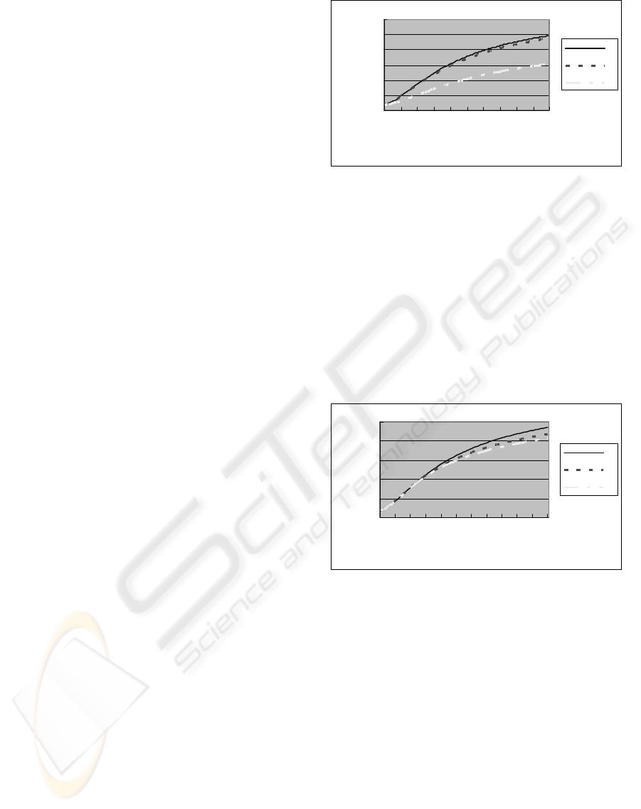
5.1 Growth Simulation of Single Tree
5.1.1 Ignore the Height Influence
According to the literature, at the age of 10, the
height of Korean pine can reach 4.2 m, DBH is
about 2.7 cm. At the age of 20, the tree height can
reach 8.6 m, DBH is about 11.9 cm. At the age of
26, the tree height can reach 10 m, DBH is about
15.5 cm. In this experiment growth of single Korean
pine is simulated in 100 years. As the DBH can be
calculated by its height based on equation (5), in
Figure 2 we only show the relationship between age
of the tree and its height. Curve A shows the
growing process of the tree at height of 0m where
the temperature is supposed to be in ideal state for
convenience. As shown in the figure, the result of
our program is close to the actual growing progress.
0
5
10
15
20
25
30
1 112131415161718191
year
height（M）
A
B
C
Figure 2: Relationship between age of the tree and its
height.
5.1.2 The Influence of Height to Tree
Growth
As in our system the height of 0m is set to be the
optimal position on temperature, so when the height
increases, the temperature decreases, then the tree
growth will be inhibited. In Figure 2 curve B and C
represent the tree growing process at the height of
100m and 300m separately. The curves show the
influence of height (or temperature) to tree growth.
0
5
10
15
20
25
1 10192837465564738291100
year
height(CM)
A
B
C
Figure 3: Growth of trees with different number of
neighbours.
5.2 Growth Simulation of Multiple
Trees
In this experiment there are 100 trees in the forest at
different positions. As trees will compete for the
limited resource, so the tree growth will be inhibited.
The more neighbors a tree has, the bigger influence
there will be to the tree growing process. In this
experiment tree regeneration and mortality are
ignored.
We chose three representative trees. In Figure 3,
curve A represent a tree has one neighbor, B has
three neighbors and C has five neighbors. As shown
in Figure 3, the influence of neighbors to the tree
growth will be bigger if it has more neighbors.
ICEIS 2009 - International Conference on Enterprise Information Systems
70

5.3 Tree Regeneration and Mortality
Taken into Consideration
As the tree growth rate, mortality, the number of
regeneration and their positions are random, every
evolve result is different, we just show one of these.
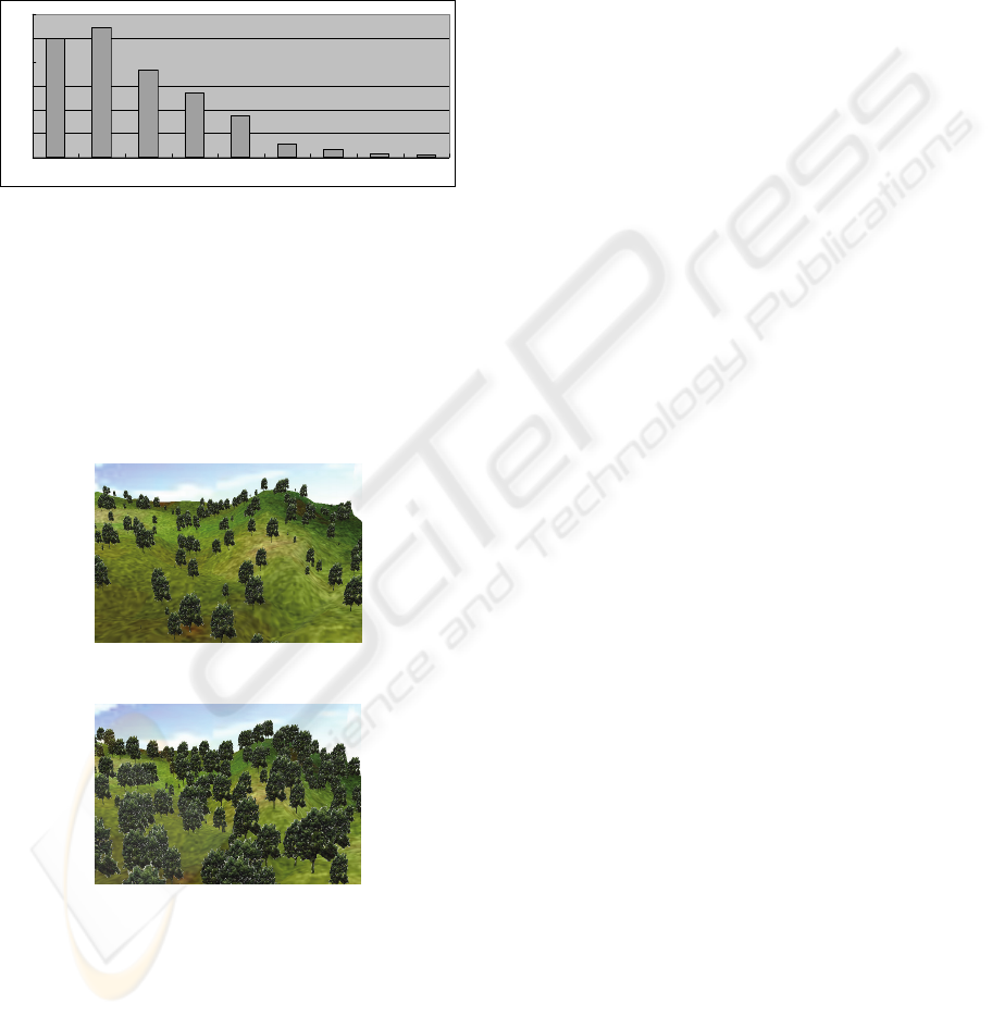
5.3.1 Proportion between Different Ages
100
109
73
54
35
11
7
3
2
0
20
40
60
80
100
120
0-20 20-40 40-60 60-80 80-100 100-120 120-140 140-160 160-180
Figure 4: Proportion between different ages.
The number of trees in forest is set to 50 initially and
it changes with trees regeneration and mortality. The
number of trees increases significantly at the
beginning, after a number of years evolving it tends
to be stable around 400. When the program
terminated there’re 394 trees in the forest. Tree
numbers of every 20 years is shown in Figure 4.
Most trees are under age of 80 and few are over 100.
Figure 5: Scene rendered at the age of 50.
Figure 6: Scene rendered at the age of 300.
5.3.2 Visualization of Trees Distribution
Based on the forest evolving result we render two
scenes at age of 50 and 300. As shown in Figure 5
and Figure 6, they’re different in tree size and dense.
6 CONCLUSIONS
We extend the forest gap model with the terrain and
the environmental factors are mapped into the tree
grow function, and then imitate the influence of
light, terrain and competition to the trees in the
forest. We implement the system with
VC++ 6.0 and
OpenGL to simulate the trees growing in forest and
the result is satisfying. The system will later be
enhanced, as it cannot imitate the competition
between different tree species, this need to be
improved later.
ACKNOWLEDGEMENTS
The research work in this paper is sponsored by
National Natural Science Foundation of China
(60773116, 60403046), National 863 High
Technology Planning of China (No. 2008AA01Z302)
and Zhejiang Natural Science Foundation of China
(Y106484, Y1080669).
REFERENCES
Lane B., Prusinkiewicz P., 2002. Generating Spatial
Distributions for Multilevel Models of Plant
Communities[J]. Graphics Interface, 69–80.
De Reffye P., Hu B. G., 2003. Relevant choices in botany
and mathematics for building efficient dynamic plant
growth models: GreenLab case[C]. In Proc. PMA03,
Beijing, 87–107.
Sang W., Ma K., Chen L., Zhen Y., 1999. A Brief Review
on Forest Dynamics Models [J]. Chinese Bulletin Of
Botany, 16(3): 193–200.
Sang W., Li J.,1998. Dynamics Modeling of Korean Pine
Forest in Southern Lesser XINGAN Mountains of
China [J]. Acta Ecologica Sinica, 18(1):38–47.
Sang W., Chen L., Ma K., 1999. Research on Succession
Medel FORPAK of Mongolian Oak-Korean Pine
Forest[J]. Acta Botanica Sinica, 41 (6) :658–668.
Prusinkiewicz P. and Lindenmayer A., 1990. The
algorithmic Beauty of Plants. Springer-Verlag. New
York.
Prusinkiewicz P., Mundermann L., Karwowski R., and
Lane B., 2001. The use of positional information in
the modeling of plants. Proceeding of SIGGRAPH
2001, 289-300.
Le Chevalier V., Jaeger M., Mei X.,Cournede P., 2007.
Simulation and visualization of functional landscapes:
Effects of the Water Resource Competition Between
Plants, Journal of Computer Science and Technology,
22(6):835-845.
SIMULATION OF FOREST EVOLUTION - Effects of Environmental Factors to Trees Growth
71