RICCATI SOLUTION FOR DISCRETE STOCHASTIC SYSTEMS
WITH STATE AND CONTROL DEPENDENT NOISE
Randa Herzallah
Faculty of Engineering Technology, Al-Balqa’ Applied University, Jordan
Keywords:
Functional uncertainties, Cautious controller, Stochastic systems, Nonlinear functions.
Abstract:
In this paper we present the Riccati solution of linear quadratic control problems with input and state dependent
noise which is encountered during our previous study to the adaptive critic solution for systems characterized
by functional uncertainty. Uncertainty of the system equations is quantified using a state and control dependent
noise model. The derived optimal control law is shown to be of cautious type controllers. The derivation of
the Riccati solution is via the principle of optimality. The Riccati solution is implemented to linear multi
dimensional control problem and compared to the certainty equivalent Riccati solution.
1 INTRODUCTION
The objective of this paper is to introduce the Ric-
cati solution of stochastic linear quadratic systems
with input and state dependent noise which is encoun-
tered during our previous study (Herzallah, 2007)
of the adaptive critic solution to stochastic systems
characterized by functional uncertainty. The prob-
lem of stochastic linear quadratic control is discussed
in (Rami et al., 2001) and is shown to have different
form than that of traditional linear quadratic control.
However, the work in (Rami et al., 2001) discusses
models with multiplicative white noise on both the
state and control and it is for continuous time sys-
tems. In the current paper the optimal control law for
stochastic discrete linear quadratic systems character-
ized by functional uncertainty will be derived. This
yields a cautious type controller which takes into con-
sideration model uncertainty when calculating the op-
timal control law.
The optimization problem of the linear stochastic
control with state and control dependent noise is to
find a feedback control which minimizes the follow-
ing quadratic cost function (Herzallah, 2007):
L =
N−
X
k=
U(x(k),u(k)) + ψ[x(N)], (1)
where
U(x(k), u(k)) = x
T
(k)Qx(k) + u
T
(k)Ru(k) (2)
ψ[x(N)] = x
T
(N)Cx(N) + Zx(N) + U

, (3)
subject to the system equation given by
x(k+ ) =
˜
Gx(k) +
˜
Hu(k) +
˜
η(k+ ), (4)
where N is the time horizon, x ∈ R
n
represents the
state vector of the system, u ∈ R
m
denotes the control
action, U(x(k), u(k)) is a utility function, ψ[(x(N) is
the weight of the performance measure due to the final
state, and
˜
η(k+) is an additive noise signal assumed
to have zero mean Gaussian distribution of covariance
matrix
˜
P. If the matrices
˜
G and
˜
H were known and
the system was noiseless, the solution of this problem
is well known (Anderson and Moore, 1971; Ogata,
1987). The optimal control is a linear function of x
which is independent of the additive noise
˜
η(k + ).
This solution is also applicable in the presence of in-
dependent noise
˜
η(k+), because the covariance ma-
trix
˜
P, of the noise term is independent of u(k).
In the current paper the optimal control for sys-
tems with unknown models will be derived. It has
been shown that systems with unknown functions
should be formulated in an adaptive control frame-
work which is known to have functional uncertain-
ties (Fel’dbaum, 1960; Fel’dbaum, 1961). This means
that state and control dependent noise always accom-
pany systems with unknown models. In the literature,
three different methods were used to handle the con-
trol problem of systems characterized by functional
uncertainty. The first method is the heuristic equiva-
lent control method (
˚
Astr¨om and Wittenmark, 1989;
Guo and Chen, 1991; Xie and Guo, 1998; Yaz, 1986)
in which the control is found by solving for the equiv-
alent deterministic system and then simply replace the
115
Herzallah R. (2009).
RICCATI SOLUTION FOR DISCRETE STOCHASTIC SYSTEMS WITH STATE AND CONTROL DEPENDENT NOISE.
In Proceedings of the 6th International Conference on Informatics in Control, Automation and Robotics - Intelligent Control Systems and Optimization,
pages 115-120
DOI: 10.5220/0002160501150120
Copyright
c
 SciTePress

unknown variables by their estimates. The second
method is the cautious control method (Goodwin and
Sin, 1984; Apley, 2004; Campi and Prandini, 2003;
Herzallah and Lowe, 2007) which takes the uncer-
tainty of the estimates into consideration when cal-
culating the control but do not plan for any probing
signals to reduce the future estimation of uncertainty.
The last but most efficient method is the dual control
method (Fel’dbaum, 1960; Fel’dbaum, 1961; Fabri
and Kadirkamanathan, 1998; Filatov and Unbehauen,
2000; Maitelli and Yoneyama, 1994) which takes un-
certainty of the estimates into consideration when es-
timating the control and at the same time plan to re-
duce future estimation of uncertainty.
The Riccati solution in this paper is for the more
general systems of equation (4), where the parameters
of the system equation are unknown and where the
noise term is state and control dependent. The param-
eters of the model are to be estimated on–line based
on some observations. Not only the model parame-
ters are to be estimated on–line, but also the state de-
pendent noise which characterizes uncertainty of the
parameters estimate and allows estimating the condi-
tional distribution of the system output or state. The
conditional distribution of the system output will be
estimated by the method used in (Herzallah, 2007).
The optimal control is again linear in x, but is now
rather critically dependent on the parameters of the
estimated uncertainty of the error
˜
η(k + ). This in
turn, yields a cautious type controller which takes into
consideration model uncertainty when calculating the
optimal control law. A numerical example is provided
and the result is compared to the certainty equivalent
controller.
The Riccati solution will be introduced soon, but
first we give a brief discussion about estimating model
uncertainty which we need for the derivation of the
Riccati solution of the cautious controller.
2 BASIC ELEMENTS
As a first step to the optimization problem, the condi-
tional distribution of the system output or state needs
to be estimated. According to theorem 4.2.1 in (Ger-
sho and Gray, 1992), the minimum mean square er-
ror (MMSE) estimate of a random vector Z given an-
other random vector X is simply the conditional ex-
pectation of Z given X ,
^
Z = E(Z | X ). For the linear
systems discussed in this paper, a generalized linear
model is used to model the expected value of the sys-
tem output,
ˆx(k + ) = Gx(k) + Hu(k) (5)
The parameters of the generalized linear model are
then adjusted using an appropriate gradient based
method to optimize a performance function based on
the error between the plant and the linear model out-
put. The stochastic model of the system of equa-
tion (4) is then shown (Herzallah, 2007) to have the
following form:
x(k+ ) = ^x(k+ ) + η(k+ ), (6)
where η(k+ ) represents an input dependent random
noise.
Another generalized linear model which has the
same structure and same inputs as that of the model
output is then used to predict the covariance matrix, P
of the error function η(k+ ),
P = Ax(k) + Bu(k). (7)
where A and B are partitioned matrices and are up-
dated such that the error between the actual covari-
ance matrix and the estimated one is minimized.
Detailed discussion about estimating the condi-
tional distribution of the system output can be found
in (Herzallah, 2007; Herzallah and Lowe, 2007).
3 RICCATI SOLUTION AND
MAIN RESULT
In this section we derive the Riccati solution of the in-
finite horizon linear quadratic control problem char-
acterized by functional uncertainty. We show here
that the optimal control law is a state feedback law
which depends on the parameters of the estimated un-
certainty, and that the optimal performance index is
quadratic in the state x(k) which also dependent on
the estimated uncertainty. The derivation is based
on the principal of optimality and is for finite hori-
zon control problem which is known to be the steady
state solution for an infinite horizon control problem.
Hence, by the principal of optimality the objective is
to find the optimal control sequence which minimizes
Bellman’s equation (Bellman, 1961; Bellman, 1962)
J[(x(k)] = U(x(k),u(k)) + γ < J[x(k+ )] >, (8)
where < . > is the expected value, J[x(k)] is the cost
to go from time k to the final time, U(x(k), u[x(k)])
is the utility which is the cost from going from time
k to time k + , and < J[x(k + )] > is assumed to
be the average minimum cost from going from time
k+  to the final time. The term γ is a discount factor
( ≤ γ ≤ ) which allows the designer to weight the
relative importance of present versus future utilities.
Using the general expressions of Equa-
tions (2), (6) and (5) in Bellman’s equation and
ICINCO 2009 - 6th International Conference on Informatics in Control, Automation and Robotics
116

taking γ = , yields
J[(x(k)] = u
T
(k)Ru(k) + x
T
(k)Qx(k) +
< J[Gx(k) + Hu(k) + η(k+ )] > . (9)
The true value of the cost function J is shown
in (Herzallah, 2007) to be quadratic with the follow-
ing form
J(x) = x
T
Mx+ Sx+ U

. (10)
Making use of this result in equation (9) yields
J[(x(k)] = u
T
(k)Ru(k) + x
T
(k)Qx(k)
+ < [Gx(k) + Hu(k) + η(k+ )]
T
M(k+ )[Gx(k) + Hu(k) + η(k+ )]
+S(k+ )[Gx(k) + Hu(k) + η(k+ )] > . (11)
Evaluating the expected value of the third term of
equation (11) and using equation (7) yields
J[(x(k)] = u
T
(k)Ru(k) + x
T
(k)Qx(k)
+ x
T
(k)G
T
M(k + )Gx(k)
+ x
T
G
T
M(k + )Hu(k)
+ u
T
(k)H
T
M(k + )Hu(k)
+ tr[AM(k + )]x(k) + tr[BM(k + )]u(k)
+ S(k+ )[Gx(k) + Hu(k)]. (12)
Minimization of the explicit performance index de-
fined in Equation (12) leads to the control law speci-
fied in the following theorem.
Theorem 1: The control law minimizing the per-
formance index J[(x(k)] of Equation (12), is given by
u
∗
= −K(k)x(k) − Z(k), (13)
where
K(k) =

R+ H
T
M(k + )H

−

H
T
M(k + )G

(14)
Z(k) =

R+ H
T
M(k + )H

−



tr[BM(k + )]
+S(k + )H

. (15)
Proof. This theorem can be proved directly by de-
riving Equation (12) with respect to the control and
setting the derivative equal to zero. Note that the opti-
mal control law consists of two terms: the linear term
in x which is equivalent to the linear term obtained in
deterministic control problems and an extra constant
term which gives cautiousness to the optimal control
law. Note also that the evaluation of the optimal con-
trol law requires evaluating the matrix, M(k + ) and
the vector, S(k + ). This evaluation can be obtained
by evaluating the optimal cost function J[(x(k)].
The optimal cost function J[(x(k)] can be obtained
by substituting Equation (13) in (12). This yields the
quadratic cost function defined in the following theo-
rem.
Theorem 2: The optimal control law defined in
Equation (13) yields a quadratic cost function of the
following form
J[(x(k)] = x
T
(k)M(k)x(k) + S(k)x(k) +U

, (16)
where
M(k) = Q+ G
T
M(k + )G
− G
T
M(k + )HF
−
H
T
M(k + )G (17)
S(k) = tr[AM(k + )] −

tr[BM(k+ )]
+ S(k + )H

F
−
H
T
M(k + )G
+ S(k + )G. (18)
and where
F
−
= [R+ H
T
M(k+ )H]
−
. (19)
Equation (17) is called the Riccati equation. It is
similar to that obtained for the certainty equivalent
controller. Equation (18) is dependent on the solu-
tion of the Riccati equation. It provides cautious-
ness to the optimal quadratic controller, therefore,
will be referred to as the equation of cautiousness.
According to equation (3), the optimal cost at k =
N equal to ψ[(x(N)]. This means that M(N) = C
and S(N) = Z. Hence equation (17) and (18) can
be solved uniquely backward from k = N to k = .
That is M(N), M(N − ), . .. , M() and S(N), S(N −
),. . ., S() can be obtained starting from M(N) and
S(N) which are known.
To reemphasize, the matrix M(k) has an equiv-
alent form similar to that obtained for deterministic
control problems. However the optimal control law
and the cost function are dependent on the values of
the vector S(k) as well as on M(k).
For infinite horizon control problems, the optimal
control solution becomes a steady state solution of
the finite horizon control (Ogata, 1987; Anderson and
Moore, 1971). Hence K(k), Z(k), M(k), and S(k) be-
come constant and defined as follows
K =

R+ H
T
MH

−

H
T
MG

(20)
Z =

R+ H
T
MH

−



[trBM] + HS

(21)
M = Q+ G
T
MG− G
T
MHF
−
H
T
MG (22)
S = tr[AM] −

tr[BM] + SH

F
−
H
T
MG
+ SG. (23)
In implementing the steady state optimal controller,
the steady state solution of the Riccati equation as
RICCATI SOLUTION FOR DISCRETE STOCHASTIC SYSTEMS WITH STATE AND CONTROL DEPENDENT
NOISE
117

well as the equation of cautiousness should be ob-
tained. Since the Riccati equation of the cautious con-
troller derived in this paper has similar form to that of
the certainty equivalent controller, standard methods
proposed in (Ogata, 1987) can be implemented to ob-
tain the solution of the Riccati equation. To obtain the
solution of the steady state equation of cautiousness
given by Equation (23),
S = tr[AM] −

tr[BM] + SH

F
−
H
T
MG+ SG,
we simply start with the non steady state equation of
cautiousness which was given by Equation (18),
S(k) = tr[AM(k+ )] −

tr[BM(k+ )]
+ S(k+ )H

F
−
H
T
M(k+ )G
+ S(k+ )G, (24)
by substituting the steady state matrix M and revers-
ing the direction of time, we modify Equation (24) to
read
S(k + ) = tr[AM] −

tr[BM]
+ S(k)H

F
−
H
T
MG+ S(k)G. (25)
Then beginning the solution with S() = 0, iterate
Equation (25) until a stationary solution is obtained.
4 SIMULATION EXAMPLE
To numerically test and demonstrate the Riccati solu-
tion of the cautious controller, the theory developed
in the previous section is applied here to 2–inputs 3–
outputs control problem described by the following
stochastic equation
x(k+ ) = Gx(k) + Hu(k) + w(k + ), (26)
where
G =


  
  
−. . 


, H =


 
 
 


,


x

()
x

()
x

()


=



−



E[w(k + )w
T
(k+ )] =


.  
 . 
  .


.
Note that although the added noise to the system of
Equation (26) is not state and control dependent, the
estimated noise is state and control dependent reflect-
ing the fact that the estimated model is not exact. The
performance index to be minimized is specified so as
to keep the state values near the origin. That is
J =
∞
X
k=
[x
T
(k)Qx(k) + u
T
(k)Ru(k)], (27)
where Q = I and R = I. Three generalized linear
models were used to provide a prediction for the
states, x

, x

and x

. The covariance matrix of the
state vector is assumed to be diagonal, therefore, one
generalized linear model with three outputs was used
to provide a prediction for the variance of the error of
estimating the first state x

, the second state x

and the
third state x

.
For comparison purposes, the optimal control law
is calculated by assuming the certainty equivalence
method where conventional Riccati solution is used
to estimate the optimal control, and by taking uncer-
tainty measure into consideration where the proposed
Riccati solution is used to estimate the optimal con-
trol. The same noise sequence and initial conditions
were used in each case. The generalized linear mod-
els were never subjected to an initial off–line train-
ing phase. Closed loop control was activated imme-
diately, with the initial parameter estimates selected
at random from a zero mean, isotropic Gaussian, with
variance scaled by the fan-in of the output units. The
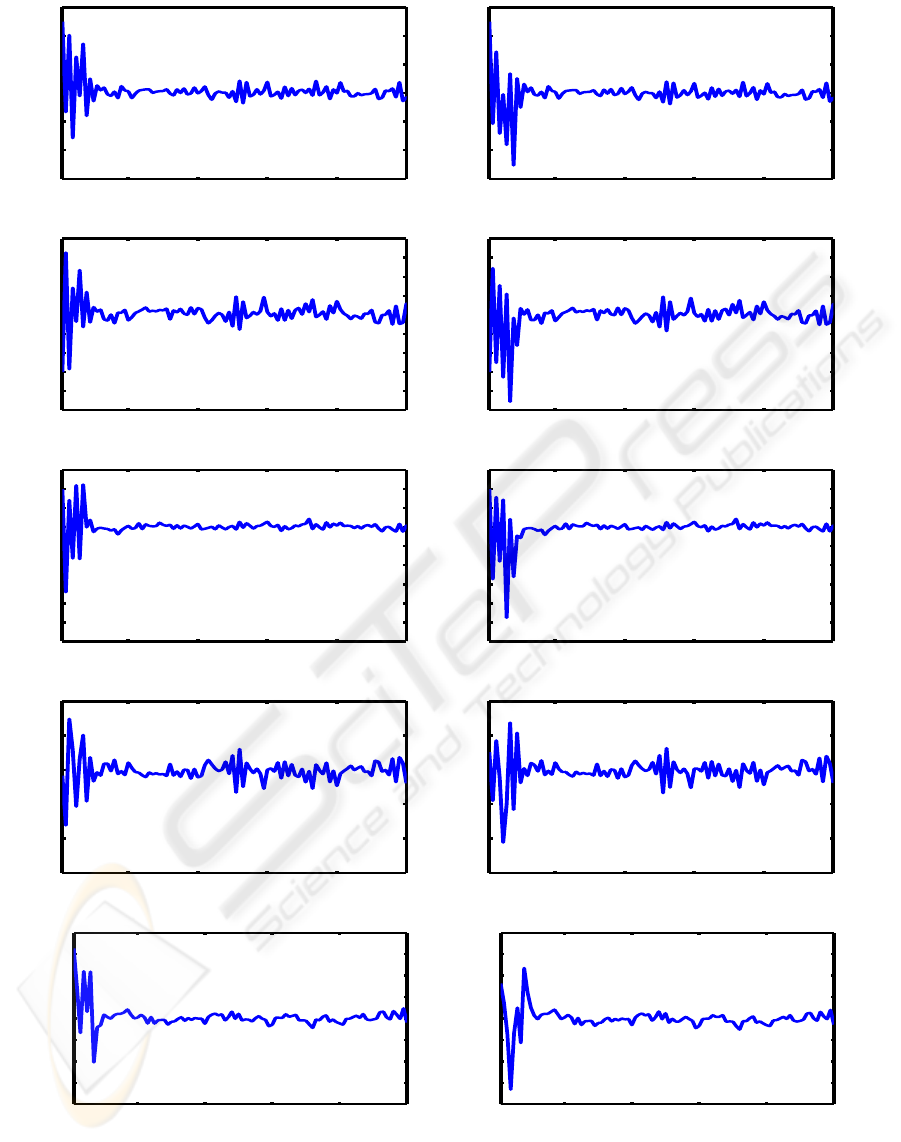
output of the two methods is shown in Figure 1. As
expected, the figure shows that the certainty equiv-
alence controller initially responds crudely, exhibit-
ing large transient overshoot because it is not taking
into consideration the inaccuracy of the parameter es-
timates. Only after the initial period, when the param-
eters of the system model converge, does the control
assume good tracking. On the other hand, the cau-
tious controller does not react hastily during the ini-
tial period, knowing that the parameters estimate are
still inaccurate.
5 CONCLUSIONS
In this paper, we have derived the Riccati solution for
more general systems with unknown functionals and
state dependent noise. The Riccati solution of this
paper is suitable for deterministic and stochastic con-
trol problems characterized by functional uncertainty.
The optimal control is of cautious type and takes into
consideration model uncertainty.
The derived Riccati equation in this paper has sim-
ilar form to that of the certainty equivalent controller.
However, as a result of considering the uncertainty on
the models, the derived optimal control law has been
ICINCO 2009 - 6th International Conference on Informatics in Control, Automation and Robotics
118

20 40 60 80 100
−6
−4
−2
0
2
4
6
Time
State x1
20 40 60 80 100
−6
−4
−2
0
2
4
6
Time
State x1
(a) (f)
20 40 60 80 100
−5
−4
−3
−2
−1
0
1
2
3
4
Time
State x2
20 40 60 80 100
−5
−4
−3
−2
−1
0
1
2
3
4
Time
State x2
(b) (g)
20 40 60 80 100
−6
−5
−4
−3
−2
−1
0
1
2
3
Time
State x3
20 40 60 80 100
−6
−5
−4
−3
−2
−1
0
1
2
3
Time
State x3
(c) (h)
20 40 60 80 100
−3
−2
−1
0
1
2
Time
Control u1
20 40 60 80 100
−3
−2
−1
0
1
2
Time
Control u1
(d) (i)
20 40 60 80 100
−2
−1.5
−1
−0.5
0
0.5
1
1.5
2
Time
Control u2
20 40 60 80 100
−2
−1.5
−1
−0.5
0
0.5
1
1.5
2
Time
Control u2
(e) (j)
Figure 1: Controlled multi dimensional stochastic system: (a) State  using the proposed Riccati solution. (b) State  using the
proposed Riccati solution. (c) State  using the proposed Riccati solution. (d) Control  using the proposed Riccati solution.
(e) Control  using the proposed Riccati solution. (f) State  using the conventional Riccati solution. (g) State  using the
conventional Riccati solution. (h) State  using the conventional Riccati solution. (i) Control  using the conventional Riccati
solution. (j) Control  using the conventional Riccati solution.
RICCATI SOLUTION FOR DISCRETE STOCHASTIC SYSTEMS WITH STATE AND CONTROL DEPENDENT
NOISE
119

shown to have an extra term which depends on the
estimated uncertainty. A simulation example has il-
lustrated the efficacy of the cautious controller.
REFERENCES
Anderson, B. D. O. and Moore, J. B. (1971). Linear Op-
timal Control. Prentice-Hall, Inc., Englewood Cliffs,
N.J.
Apley, D. (2004). A cautious minimum variance con-
troller with ARIMA disturbances. IIE Transactions,
36(5):417–432.
˚
Astr¨om, K. J. and Wittenmark, B. (1989). Adaptive Control.
Addison-Wesley, Reading, MA, U.S.A.
Bellman, R. E. (1961). Adaptive Control Processes. Prince-
ton University Press, Princeton, NJ.
Bellman, R. E. (1962). Applied Dynamic Programming.
Princeton University Press, Princeton, NJ.
Campi, M. C. and Prandini, M. (2003). Randomized al-
gorithms for the synthesis of cautious adaptive con-
trollers. Systems and Control Letters, 49:21–36.
Fabri, S. and Kadirkamanathan, V. (1998). Dual adaptive
control of nonlinear stochastic systems using neural
networks. Automatica, 34(2):245–253.
Fel’dbaum, A. A. (1960). Dual control theory I-II. Automa-
tion and Remote Control, 21:874–880.
Fel’dbaum, A. A. (1961). Dual control theory III-IV. Au-
tomation and Remote Control, 22:109–121.
Filatov, N. M. and Unbehauen, H. (2000). Survey of adap-
tive dual control methods. IEE Proceedings Control
Theory and Applications, 147:118–128.
Gersho, A. and Gray, R. M. (1992). Vector Quantization
and Signal Compression. Kluwer Academic Publish-
ers.
Goodwin, G. C. and Sin, K. S. (1984). Adaptive Filter-
ing Prediction and Control. Prentice-Hall, Englewood
Cliffs, NJ.
Guo, L. and Chen, H.-F. (1991). The
˚
Astr¨om–Wittenmark
self–tuning regulator revisited and ELS–based adap-
tive trackers. IEEE Transactions on Automatic Con-
trol, 36(7):802–812.
Herzallah, R. (2007). Adaptive critic methods for stochas-
tic systems with input-dependent noise. Automatica,
43(8):1355–1362.
Herzallah, R. and Lowe, D. (2007). Distribution model-
ing of nonlinear inverse controllers under a Bayesian
framework. IEEE Transactions on Neural Networks,
18:107–114.
Maitelli, A. L. and Yoneyama, T. (1994). A two stage
suboptimal controller for stochastic systems using ap-
proximate moments. Automatica, 30(12):1949–1954.
Ogata, K. (1987). Discrete Time Control Systems. Prentice
Hall, Inc., EnglewoodCliffs, New Jersey.
Rami, M. A., Chen, X., Moore, J. B., and Zhou, X. Y.
(2001). Solvability and asymptotic behavior of gner-
alized riccati equations arising in indefinite stochastic
lq controls. IEEE Transactions on Automatic Control,
46(3):428–440.
Xie, L. L. and Guo, L. (1998). Adaptive control of a class
of discrete time affine nonlinear systems. Systems and
Control Letters, 35:201–206.
Yaz, E. (1986). Certainty equivalent control of stochastic
sytems: Stability property. IEEE Transactions on Au-
tomatic Control, 31(2):178–180.
ICINCO 2009 - 6th International Conference on Informatics in Control, Automation and Robotics
120