MOBILE PLATFORM SELF-LOCALIZATION IN PARTIALLY
UNKNOWN DYNAMIC ENVIRONMENTS
Patrice Boucher, Sousso Kelouwani and Paul Cohen
Perception and Robotics Laboratory, Ecole Polytechnique de Montreal
2500, Chemin de Polytechnique, Montreal, Canada
Keywords:
Navigation, Localization, Dynamic environments, Point-based model, Extended Kalman Filter, 2D Point
matching, Registration, Robotic platform slipping, Homogeneous matrices.
Abstract:
Localization methods for mobile platforms are commonly based on an observation model that matches onboard
sensors measures and environmental a priori knowledge. However, their effectiveness relies on the reliability
of the observation model, which is usually very sensitive to the presence of unmodelled elements in the en-
vironment. Mismatches between the navigation map, itself an imperfect representation of the environment,
and actual robot’s observations introduce errors that can seriously affect positioning. This article proposes
a 2D point-based model for range measurements that works with a new method for 2D point matching and
registration. The extended Kalman filter is used in the localization process since it is of the most efficient
tool for tracking a robotic platform’s configuration in real time. The method minimizes the impact of mea-
surement noise, mismodelling and skidding on the matching procedure and allows the extended Kalman filter
observation model to be robust against skidding and unmodelled obstacles. Its O(n · m) complexity enables
real-time optimal points matching. Simulation and experiments demonstrate the effectiveness and robustness
of the proposed algorithm in dynamic and partially unknown environments.
1 INTRODUCTION
In the context of map-based navigation, a robotic plat-
form must regularly and reliably estimate its configu-
ration (position and orientation) within a known map
of the environment. This problem is commonly re-
ferred to as the localization problem. By knowing its
configuration and perceiving obstacles in the environ-
ment, the platform can choose appropriate actions in
order to reach a given destination. However, moving
efficiently requires an accurate localization method
combined with fast real-time sensory data processing.
The proposed algorithm in this paper fulfills these two
requirements, using extended Kalman filtering with a
novel observation model for platform localization.
Proposed by Stanley F. Schmidt in 1970 (Schmidt,
1970), the extended Kalman filter is commonly used
for parameters estimation with non linear models sub-
ject to noise. The Kalman filter computes a config-
uration estimate in two steps. The first one is the
prediction step, based on the dynamic model of the
system. The second step, known as the correction
step, is based on an observationmodel that draws rela-
tionships between the platform configuration and key
measurements. In indoor environments, the localiza-
tion of a robotic platform is often based on obser-
vations provided by on-board sensors such as laser
range finder (Carlson et al., 2008), infrared sensor
(Wei et al., 2005) and sonar sensors. Observed fea-
tures are matched with a priori data about the envi-
ronment in order to estimate the most plausible plat-
form’s configuration.
As explained in (Thrun et al., 2005) and (De Laet
et al., 2008), the matching process from range
finder data can be addressed with beams-based mod-
els, feature-based methods and correlation-based ap-
proaches. In order to deal with unmodelled objects,
the beams-based and correlation-based approaches
compute complex probabilistic functions given the a
priori knowledge about the navigation environment
(De Laet et al., 2008). Since each range measurement
is considered separately, such models do not take ad-
vantageof the natural features of the surrounding plat-
form area. On the other hand, despite that feature-
based models can be robust against unexpected ob-
jects through selectivity, feature extraction and recog-
113
Boucher P., Kelouwani S. and Cohen P.
MOBILE PLATFORM SELF-LOCALIZATION IN PARTIALLY UNKNOWN DYNAMIC ENVIRONMENTS.
DOI: 10.5220/0002162001130120
In Proceedings of the 6th International Conference on Informatics in Control, Automation and Robotics (ICINCO 2009), page
ISBN: 978-989-674-000-9
Copyright
c
 2009 by SCITEPRESS – Science and Technology Publications, Lda. All rights reserved

nition may be computationally expensive and the fea-
tures must be sufficiently distinctive and numerous.
The lack of robustness of observation models against
unmodelled objects is usually compensated by adding
such objects onto the map through simultaneous lo-
calization and map building (SLAM). However, it re-
mains attractive to have at the base a robust obser-
vation model without map modification for avoiding
complications at upper levels.
For these reasons, we introduce in this paper a 2D
point-based approach which works with a local occu-
pancy grid-map instead of using direct sensor mea-
surements or high level features. In this way, the as-
sociation process is made between a set of points, ex-
tracted from the measurements, with a second set ex-
tracted from the grid-map. The configuration is then
deduced by matching both sets. Two-dimensional
point matching involves two main issues : pairing two
sets of 2D points and geometrical matching. The most
commonly used methods for geometric matching in-
clude SVD (Singular Value Decomposition) (Arun
et al., 1987), unit quaternions methods (Horn, 1987)
and double quaternionsmethods (Walker et al., 1991).
Various approaches also solve the problem of pair-
ing and matching simultaneously. Many of them are
based on iterative algorithms as in (Zhang, 1994) and
(Ho et al., 2007). Moreover, (Censi et al., 2005) pro-
poses a Hough Scan Matching (HSM) approach based
on the Hough Transform. However, these approaches
do not explicitly mention the matching error in the
mathematical formulation, a fact that cause ambiguity
in the accurate evaluation of the homogeneous matri-
ces. Since the approach presented in this paper needs
robustness against matching errors caused by unmod-
elled objects, these methods are not convenient for a
robust 2D points observation model.
In summary, the main contributions of this paper
are: (1) a fast method of 2D points registration with
complexity O(n· m) (O(n) for the geometric match-
ing) that takes into account the presence of matching
errors and measurement noise for enabling realistic
accuracy evaluation of the homogeneous matrices; (2)
a simple and fast 2D point-based observation model
that works in presence of unmodelled objects (3) a
novel method for robotic platform localization based
upon extended Kalman filtering. The rest of the pa-
per is organized in five sections. Section 2 presents a
mathematical formulation of the problem. In section
3, a new method for finding 2D homogeneous ma-
trices is presented. In section 4, we present how the
overall methodology can be combined with extended
Kalman filtering for platform localization. Section 5
presents and discusses experimental results.
2 PROBLEM STATEMENT
The dynamic equation of a robotic platform moving
in a 2D plan can be represented at each instant k by :
X
k+1
= f(X
k
,V
k
) + ψ
k
where X
k
is the platform state variable at instant k,
V
k
is the speed of the platform at instant k, ψ
k
is the
uncertainty (noise) on the dynamic model and f(.,.)
is the function used to compute the predicted state.
The observation model is represented by:
Z
k
= h(X
k
) + ξ
k
where Z
k
represents the observations by the platform
sensors, ξ
k
is the uncertainty (noise) on sensor obser-
vations and h(.) is the function used to get observa-
tions when the platform is in state X
k
.
In real applications, f and h are non linear. In
order to apply Kalman filtering, the Jacobean of f and
h are computed over a nominal path. Furthermore, the
following assumptions must hold:
1. ψ
k
is uncorrelated with the state initial estimate;
2. ψ
k
and ξ
k
are uncorrelated;
3. ψ
k
and ξ
k
are zero mean random process.
Some of these assumptions may not hold if the fol-
lowing conditions occur during platform motion:
• The observations are disturbed by unmodelled ob-
stacles;
• The platform slips on the floor.
The aim is to find an observation model that reduces
significantly the impact of the platform slipping and
the presence of unmodelled obstacles.
3 FINDING OPTIMAL
HOMOGENEOUS
TRANSFORMATION
MATRICES
In this section, we present a generic method for find-
ing homogeneous transformation matrices between
two sets of 2D points.
3.1 Problem Definition
Assume 2 sets P and Q of 2D points. Assume that X
k
is the state vector of the platform at time k represent-
ing its configuration in the navigation environment. P
is the set of points measured by the platform sensors
at configuration X
k
and Q is the set of points given by
ICINCO 2009 - 6th International Conference on Informatics in Control, Automation and Robotics
114

the navigation map at that configuration. P and Q are
called real set and virtual set, respectively:
P = {p
i
,i = 1,...,N} (1)
Q = {q
i
,i = 1,...,N} (2)
We suppose that each pair {p
i
, q
i
} corresponds to
a single physical point in the environment. We also
assume that q
i
is obtained by applying the homoge-
neous transformation (T, R) on p
i
, where T is a trans-
lation vector and R is the rotation matrix.
q
i
= T + Rp
i
∀i ∈ {1,...,N} (3)
In the context of platform navigation with on-
board sensors, the set P is affected by measurement
noise. Furthermore, the real correspondence between
real and virtual points is unknown. We call
˜
P the set
of noisy measurement and
˜
Q the set of virtual points
obtained from the map and affected by pairing error:
˜
P = { ˜p
i
,i = 1,...,N}
˜
Q = { ˜q
i
,i = 1,...,N}
Representing by δ
M
i
the measurement error on p
i
and by δ
C
i
the pairing error affecting {p
i
,q
i
}, the fol-
lowing expressions can be written :
˜p
i
= p
i
+ δ
M
i
∀i ∈ {1,...,N} (4)
˜q
i
= q
i
+ δ
C
i
∀i ∈ {1,...,N} (5)
Pluggins these equations back into equation (3) yields
to the expression of the pairing error δ
C
i
:
δ
C
i
= −T −R

˜p
i
− δ
M
i

+ ˜q
i
∀i ∈ {1, . . . , N} (6)
3.2 Computing the Homogeneous
Transformation Matrices
The following assumptions are made:
1. The measurement noise and pairing error are
gaussian processes with zero mean and variance
σ
2
M
and σ
2
C
respectively:
δ
M
i
−→ N(0,σ
2
M
)
δ
C
i
−→ N(0,σ
2
C
)
2. No {R,T} other than {R
∗
,T
∗
} minimizes the
quadratic paring error.
3. The expectation of a random variable tends to be
equal to its sampling average:
χ
i
= E [χ
i
] =
1
N
N
∑
i
χ
i
Finding T
∗
as Function of R
∗
Inserting expressions (4) and (5) in (3), the translation
vector
˜
t
i
is given by:
˜
t
i
= T
∗
+ δ
C
i
− R
∗
δ
M
i
(7)
= ˜q
i
− R
∗
˜p
i
(8)
and its expectation is :
E[
˜
t
i
] = T
∗
=
˜q
i
− R
∗
˜p
i
(9)
Finding R
∗
From equation (7), the expression δ
C
i
is computed as
a function of T
∗
and R
∗
:
δ
C
i
=
˜
t
i
− T
∗
+ R
∗
δ
M
i
(10)
R
∗
and T
∗
must minimize the quadratic pairing error,
therefore:
J
∗
= minE

(δ
C
i
)
T
δ
C
i

(11)
By putting equation (10) in (11), replac-
ing E[(δ
M
i
)
T
δ
M
i
] by σ
2
M
and noticing that
E[(δ
C
i
)
T
R
∗
δ
M
i
] = σ
2
M
since δ
C
i
and δ
M
i
are corre-
lated via (10), the following expression is obtained:
J
∗
= E

(
˜
t
i
− T
∗
)
T
(
˜
t
i
− T
∗
)

− σ
2
M
(12)
This result shows that the variance of the transla-
tion vector
˜
t
i
, defined by ∆T
2
, is equal to the sum of
the minimum paring error variance and the measure-
ment noise variance :
∆T
2
= E

(
˜
t
i
− T
∗
)
T
(
˜
t
i
− T
∗
)

= E

(δ
C
i
)
T
δ
C
i

+ σ
2
M
(13)
By plugging expressions (7) and (9) into (13), and
by using the angle, φ
∗
, associated with the rotation
matrix R
∗
, the expression of the cost function can be
rewritten as :
J
∗
=
˜q
T
i
˜q
i
+ ˜p
T
i
˜p
i
− ˜q
T
i
˜q
i
− ˜p
T
i
˜p
i
− σ
2
M
(14)
−2cos(φ
∗
)

˜p
ix
˜q
ix
+ ˜p
iy
˜q
iy
− ˜p
ix
˜q
ix
− ˜p
iy
˜q
iy

−2sin(φ
∗
)

˜p
iy
˜q
ix
− ˜p
ix
˜q
iy
− ˜p
ix
˜q
iy
+ ˜p
iy
˜q
ix

where ˜p
i
= [ ˜p
ix
˜p
iy
]
T
and ˜q
i
= [ ˜q
ix
˜q
iy
]
T
. Taking
the derivative to be equal to zero, we obtain:
φ
∗
= atan2

˜p
ix
˜q
iy
− ˜p
iy
˜q
ix
− ˜p
ix
˜q
iy
+ ˜p
iy
˜q
ix
,
˜p
ix
˜q
ix
+ ˜p
iy
˜q
iy
− ˜p
ix
˜q
ix
− ˜p
iy
˜q
iy

(15)
The optimal rotation matrix can be deduced directly
from this expression. Knowing R
∗
, we can find T
∗
by
using equation (9).
MOBILE PLATFORM SELF-LOCALIZATION IN PARTIALLY UNKNOWN DYNAMIC ENVIRONMENTS
115

Algorithm
1. Compute :
˜p
ix
˜q
iy
, ˜p
iy
˜q
ix
, ˜p
ix
˜q
ix
, ˜p
iy
˜q
iy
,
˜p
ix
, ˜p
iy
, ˜q
ix
, ˜q
iy
2. Find the angle φ
∗
by using equation (15) ;
3. Compute the rotation matrix R
∗
(φ
∗
) ;
4. Compute the translation vector T
∗
(9).
3.3 Evaluation of the Algorithm
Complexity
The first step of the algorithm is related to the compu-
tation of averages. These operations have a complex-
ity O(n). Steps 2, 3 and 4 are not dependent upon data
size. Hence, the overall complexity is O(n).
3.4 Quality of the Homogeneous
Transformation Estimation
In order to assess the quality of the result, the accu-
racy of the optimal translation T
∗
and angular error
φ
∗
must be estimated for ∆T and ∆φ
∗
. These val-
ues are indispensable for estimating the measurement
noise matrix of the Kalman Filter and (if used with
Correlation-based approaches) for providing a corre-
lation measure between the both point sets, since ∆T
and ∆φ
∗
increase accordingly to the inconsistency be-
tween sets by taking into account the matching error
expectation.
Translation Vector Covariance Matrix
The covariance of the translation vector, Ω
2
T
, is de-
fined as :
Ω
2
T
= E
h
(
˜
t
i
− T
∗
)(
˜
t
i
− T
∗
)
T
i
(16)
and can be expressed as:
Ω
2
T
=

σ
2
x
σ
x
σ
y
σ
y
σ
x
σ
2
y

(17)
The covariance matrix of the translation error cor-
responds to the covariance of the pairing error added
to the covariance of the measurement noise reoriented
so as to minimize the covariance of the translation
vector, as followed :
Ω
2
T
= E

δ
C
i
(δ
C
i
)
T

+ R
∗
E

δ
M
i
(δ
M
i
)
T

(R
∗
)
T
(18)
Orientation Estimation Quality
Unlike for the translation, there is only one optimal
rotation matrix for all pairs of 2D point. Moreover, as
the optimal orientation minimizes ∆T, we can use ∆T
to assess the orientation accuracy with an empirical
formula. Considering that the maximum error of the
angle is ±π, we have:
lim
∆T→0
∆φ
∗
= 0 (19)
lim
∆T→∞
∆φ
∗
= π (20)
The following empirical formula provides a reason-
able estimate of the angle accuracy :
∆φ
∗
=
π∆T
∆T + ∆T
hight
(21)
where ∆T
hight
is a large translation error necessarily
involving bad pairing.
3.5 Robustness Improvement
The previous results are based upon the assumption
that the average pairing error is null and that the par-
ing and measurement error are gaussian process. In
particular, the presence of unknown elements in the
environment entails a systematic pairing error with a
non-zero average. Therefore the gaussien process as-
sumption may not hold. Nevertheless, assuming that
the proportion of unknown object points is low, equa-
tion (6) gives a good approximation of the correlation
error for each pair.
In this way, it is reasonable to give more weight to
pairs whose pairing error expectation δ
C
is lower. To
do this, we compute as first step, the transformation
matrices that minimize the overall expectation of pair-
ing error by using equations (15) and (9). Then, the
correlation error of each pair can be estimated through
(6), which, ignoring the measurement noise, leads to:
˜
δ
c
i
= −T
∗
− R
∗
˜p
i
+ ˜q
i
∀i ∈ {1··· , N}
From this result, an uncertainty coefficient can be de-
rived as:
(σ
c
i
)
2
=
˜
δ
c
i
∗
˜
δ
c
i
(22)
The weight, γ
i
, of each pair can then be defined as:
γ
i
(σ
c
i
) = exp{−β(σ
c
i
)
2
} (23)
where the parameter β, which can be set empirically,
determines the rejection rate for erroneouspairs. With
appropriate β, this expression allows good weighting
distribution among pairs .
Next, R
∗
and T
∗
can be updated by minimizing
the weighted paring error expectation. The solution is
identical to the one presented at (3.2), except that the
ICINCO 2009 - 6th International Conference on Informatics in Control, Automation and Robotics
116

following weighted averages are used at steps 1 and
2:
˜p
ix
˜q
iy
γ
i
, ˜p
iy
˜q
ix
γ
i
, ˜p
ix
˜q
ix
γ
i
, ˜p
iy
˜q
iy
γ
i
,
˜p
ix
γ
i
, ˜p
iy
γ
i
, ˜q
ix
γ
i
, ˜q
iy
γ
i
3.6 Algorithm Summary
From a real points set
˜
P = { ˜p
i
,i = 1,...,N} with
M candidates for each real point, such as C
i
=

c
ij
, j = 1,...,M

, find a set
˜
Q = { ˜q
i
,i = 1,...,N}
that depicts the same physical points of the environ-
ment linked to the navigation map.
Then,
1. Choose the nearest neighbour of set P :
˜q
i
= arg min
1≤ j≤M
dist ( ˜p
i
,c
ij
)
where dist is the Euclidean distance.
2. Find R
∗
and T
∗
by geometric matching (3.2).
3. Weighting each pair with (23), recalculate R
∗
and
T
∗
with weighting averages (see 3.5).
Algorithm Complexity
In sub-section (3.3), we showed that geometric
matching is of O(n) complexity. As each additional
point involves M extra comparisons, then the com-
plexity of step 1 is directly proportional to the number
of points. Therefore, this step is complexity O(n· m).
Step 3 involves one weight computation per point, so
the complexity is O(n). Hence, the total method re-
mains complexity O(n· m).
4 EXTENDED KALMAN FILTER
FOR LOCALIZATION
In this section, we demonstrate how the proposed
points matching method can be used to enhance the
robustness of platform localization based on extended
Kalman filter.
4.1 Platform Dynamic Model
The platform dynamic model is usually obtained by
using the dead reckoning. Assume that [x
k
,y
k
,θ
k
]
′
,
v
k
and ω
k
represent respectively the configuration X
k
,
the translation speed and the angular speed at time k.
Assume that the integration constant step (which is
also the sampling period) is δt. We can then write the
following dynamic equations:
θ
k+1
= θ
k
+ δtω
k
x
k+1
= x
k
+ v
k
δtcosθ
k
y
k+1
= y
k
+ v
k
δtsinθ
k
It must be noted that the dynamic equation may
change according to the choice of platform model.
This is not an issue of the proposed approach since
this methodology focuses only on the observation
model of the Kalman theory.
4.2 2D Point-based Observation Model
This simplest observation model that could be used in
conjunction with Kalman filtering is represented by
the following expression:


x
k|k
y
k|k
θ
k|k


=


x
k|k−1
+ T
∗
x
y
k|k−1
+ T
∗
y
θ
k|k−1
+ φ
∗


(24)
where {x
k|k−1
,y
k|k−1
,θ
k|k−1
} is the configuration of
the platform in the navigation map coordinate sys-
tem, given all observations up to time k − 1 and
{x
k|k
,y
k|k
,θ
k|k
} is the correction based on optimal ho-
mogeneous transformation parameters, {T
∗
x
,T
∗
y
,φ
∗
},
obtained at time k. The measurement noise covari-
ance matrix is obtained by using equations (17) and
(21)
Ξ =


σ
2
x
+ ε σ
x
σ
y
0
σ
y
σ
x
σ
2
y
+ ε 0
0 0 ∆φ
∗
2
+ ε


(25)
where the added ε is required in order to keep the filter
stable when the value of the translation vector covari-
ance and the uncertainty on the estimated angle are
too small. If points are defined in the robot reference
frame, transformation matrices to convert them into
the map frame must be applied.
When the presence of a large obstacle or multi-
ples unknown obstacles results in severe erroneous
pairings between sets P and Q, the elements on the
diagonal of the noise covariance matrix Ξ increase
accordingly (see expression 18 ). This will reduce
the confidence in the observation model and increase
the confidence in the dynamic model. The impact on
the configurationestimate will be limited providedthe
disturbance is not too prolonged. Otherwise, bad ob-
servations can cause, with time, the divergence of fil-
ter. The combination large unknown obstacle - no rel-
ative motion is the worst situation for the localization
system.
MOBILE PLATFORM SELF-LOCALIZATION IN PARTIALLY UNKNOWN DYNAMIC ENVIRONMENTS
117

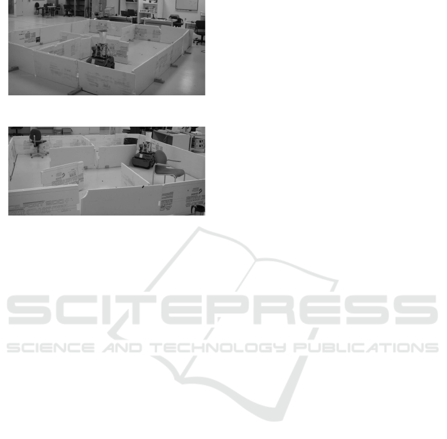
Figure 1: Controlled Navigation Environment.
Figure 2: Controlled Navigation Environment with Unmod-
elled Obstacles.
5 EXPERIMENTAL RESULTS
5.1 Experimentation Setup
Hardware and Software
The approach described in this paper has been
implemented in C++ and many simulations have
been performed in Matlab and Acropolis (Zalzal,
2006). For real experiments, Acropolis and Player-
Stage(Matthias Kranz and Schmidt, 2006) have been
used as the robotic framework. The mobile platform
hardware is an iRobot Mini ATRV with a differen-
tial driving mode and it is equiped on the front with
a Sick LMS-200 laser range finder. Laser range data
has been down-sampled in order to provide 18 mea-
surements per scan.
Navigation Environment
In order to assess the proposed methodology, a navi-
gation environment has been built. The workspace is
delimited by walls as shown on Figure (1). A map of
this environment is stored on the platform on-board
computer. Figure (2) shows the same navigation en-
vironment with additional unmodelled obstacles.
Localization Parameter Settings
• The typical noise magnitude on the translation
and angular speeds are set empirically to 0.06m/s,
and 0.06rad/s respectively. Note that this noise
is inflated in order to reduce the negative im-
pact of slippage on the platform dynamic model.
Since this noise reflects confidence toward the dy-
namic system, an inflated noise magnitude value
increases the confidence toward the observation
model. In situations where the platform is resis-
tant to slippage, the dynamic model is unbiased
and in this case a realistic estimate of noise gives
better results.
• The rejection rate β of erroneously paired points,
used in equation (23), is set empirically to 0.3.
• The value of the parameter ε, used for numerical
stability of equation (25), is set to 0.0001.
External Platform Localization System
In order to obtain an accurate estimate of the platform
position in the navigation environment, a second laser
range finder, mounted on a fix platform is used. This
device detects only the top part of the robotic plat-
form. The positions given by this range finder are
used to track the actual trajectory of the platform in
the map.
5.2 Simulation for Complexity
Assessment
Assessment of the pairing and registration approaches
has been realized using Matlab simulation. The goal
of the simulation is to find the optimal homogeneous
transformation matrices corresponding to two sets of
2D points.
The size of the sets is increased from 2
2
to 2
15
and set is randomly generated. Given T = [2 4]
′
and φ = 0.333 rad, the Q set is generated by applying
this transformation matrices to set P. Using the pro-
posed approach, given only P and Q-sets, one should
recover exact values of R and T.
Figure (3) plots the execution time as a function
of the set size. The average error on the estimation
of T
∗
and φ
∗
is 4.5926e
−15
and 3.2937e
−16
respec-
tively. Furthermore, the figure shows that there is a
linear relationship between the set size and the exe-
cution time. This result reinforces the claim that the
proposed matching method is of complexity O(n).
5.3 Experimental Tests
With the same geometrical trajectory executed repeat-
edly, the average tracking error is 0.12m with a stan-
dard deviation of 0.10m. A typical result is illustrated
on Figure (4). The solid line represents the trajectory
ICINCO 2009 - 6th International Conference on Informatics in Control, Automation and Robotics
118

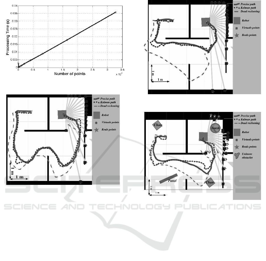
Figure 3: Processing Time as a Function of Data Size.
Figure 4: Configuration Tracking in The Navigation Envi-
ronment.
of the platform reported by the external laser range
finder. The dotted line is the trajectory computed by
using the approach described in the paper. The dashed
line corresponds to navigation with dead reckoning
only.
Figure (5) shows an example of severe slippage of
the platform during the first quarter of the trajectory.
This slippage causes an increasing deviation between
the actual trajectory, as reported by the external range
finder, and the estimated trajectory based upon dead
reckoning. By using the proposed observation model,
our estimation is similar to what has been reported by
the external range finder.
For the last scenario, several unknown obstacles
(unmodelled objects in the navigation map) have been
added in the environment. The same geometrical tra-
jectory has been executed repeatedly. As long as the
number of observed points corresponding to unknown
obstacles remains smaller that the number of points
from the known environment, the estimated position
of the platform as reported by the approach is still rea-
sonably good. Figure (6) shows a successful case of
path following while Figure (7) illustrates a failure of
the recovery method. In order to trigger this failure
Figure 5: Configuration Tracking with Platform Slipping.
Figure 6: Configuration Tracking with Platform Slipping
and Unknown Obstacles.
situation, the robot was forced to remain stationary in
front of a large unknown obstacle so that the propor-
tion of perceived 2D points from the obstacle become
preponderant for a long duration. As such contexts
normally involves important mismatches between the
two point sets, the measurement noise covariance ma-
trix (equation 25) should increase accordingly, giv-
ing priority to the dynamic model. Hence, such un-
modelled objects should hardly cause the divergence
when the platform moves continuously. Neverthe-
less, despite that this paper focuses on the localiza-
tion method without addressing the map building, this
kind of failures could be avoided by adding such ob-
jects on the map and the general accuracy of the con-
figuration estimate should also get increased.
6 CONCLUSIONS
This article has presented a fast 2D points matching
and registration algorithm of complexity O(n· m) that
MOBILE PLATFORM SELF-LOCALIZATION IN PARTIALLY UNKNOWN DYNAMIC ENVIRONMENTS
119

Figure 7: Configuration Tracking Failure.
exhibits robustness against erroneous point pairings.
We have shown that this algorithm is easily integrable
in a 2D point-based observation model for estimat-
ing a platform configuration. When used for robotic
platform localization based on extended Kalman fil-
tering, the algorithm provides an accurate estimate
of the platform configuration, even in the presence
of skidding and unknown obstacles in the environ-
ment. The observation model developed in this paper
could be used in conjunction with other localization
approaches, such as Particle Filter and Monte Carlo
filtering.
ACKNOWLEDGEMENTS
This work has been supported by the Natural Sci-
ence and Engineering Council of Canada (NSERC)
through Grant No. CRD 349481-06. The authors
wish to acknowledgethe contribution of severalmem-
bers of the Perception and Robotics Laboratory dur-
ing implementation and testing, H. Nguyen, V. Zalzal
and R. Gava.
REFERENCES
Arun, K., Huang, T., and Blostein, S. (Sept. 1987). Least-
squares fitting of two 3-d point sets [computer vision].
IEEE Transactions on Pattern Analysis and Machine
Intelligence, PAMI-9(5):698 – 700.
Carlson, J., Thorpe, C., and Duke, D. L. (2008). Ro-
bust real-time local laser scanner registration with un-
certainty estimation. Springer Tracts in Advanced
Robotics, 42:349 – 357.
Censi, A., Iocchi, L., and Grisetti, G. (2005). Scan match-
ing in the hough domain. In Robotics and Automation,
2005. ICRA 2005. Proceedings of the 2005 IEEE In-
ternational Conference on, pages 2739–2744.
De Laet, T., De Schutter, J., and Bruyninckx, H. (2008).
A Rigorously Bayesian Beam Model and an Adaptive
Full Scan Model for Range Finders in Dynamic Envi-
ronments. Journal of Artificial Intelligence Research,
33:179–222.
Ho, J., Yang, M.-H., Rangarajan, A., and Vemuri, B. (2007).
A new affine registration algorithm for matching 2d
point sets. Proceedings - IEEE Workshop on Applica-
tions of Computer Vision, WACV 2007.
Horn, B. (1987). Closed-form solution of absolute orien-
tation using unit quaternions. Journal of the Opti-
cal Society of America A (Optics and Image Science),
4(4):629 – 42.
Matthias Kranz, Radu Bogdan Rusu, A. M. M. B. and
Schmidt, A. (2006). A player/stage system for
context-aware intelligent environments. To appear
in Proceedings of the System Support for Ubiquitous
Computing Workshop, at the 8th Annual Conference
on Ubiquitous Computing (Ubicomp 2006).
Schmidt, S. F. (1970). Computational techniques in kalman
filtering. NATO Advisory Group for Aerospace Re-
search and Development.
Thrun, S., Burgard, W., and Fox, D. (2005). Probabilis-
tic Robotics (Intelligent Robotics and Autonomous
Agents). The MIT Press.
Walker, M., Shao, L., and Volz, R. (1991). Estimating 3-
d location parameters using dual number quaternions.
CVGIP: Image Understanding, 54(3):358 – 67.
Wei, P., Xu, C., and Zhao, F. (2005). A method to locate
the position of mobile robot using extended kalman
filter. Lecture Notes in Computer Science (includ-
ing subseries Lecture Notes in Artificial Intelligence
and Lecture Notes in Bioinformatics), 3801 NAI:815
– 820.
Zalzal, V. (2006). Localisation mutuelle de plates-formes
robotiques mobiles par vision omnidirectionnelle et
filtrage de Kalman. PhD thesis, Ecole Polytechnique
Montreal (Canada).
Zhang, Z. (1994). Iterative point matching for registration
of free-form curves and surfaces. International Jour-
nal of Computer Vision, 13(2):119 – 152.
ICINCO 2009 - 6th International Conference on Informatics in Control, Automation and Robotics
120