HIGHER ORDER SLIDING MODE CONTROL FOR CONTINUOUS

TIME NONLINEAR SYSTEMS BASED ON OPTIMAL CONTROL

Zhiyu Xi and Tim Hesketh

School of Electrical Engineering & Telecommunications, University of New South Wales, Kensington, NSW, Australia

Keywords:

Sliding mode, High order, Nonlinear, Optimal control.

Abstract:

This paper addresses higher order sliding mode control for continuous nonlinear systems. We propose a new

method of reaching control design while the sliding surface and equivalent control can be designed conven-

tionally. The deviations of the sliding variable and its high order derivatives from zero are penalized. This is

realized by minimizing the amplitudes of the higher order derivatives of the sliding variable. An illustrative

example— a ﬁeld-controlled DC motor— is given at the end.

1 INTRODUCTION

Variable structure systems (VSS) have been exten-

sively used for control of dynamic industrial pro-

cesses. The essence of variable structure control

(VSC) is to use a high speed switching control scheme

to drive the plant’s state trajectory onto a speciﬁed

and user chosen surface in the state space which is

commonly called the sliding surface or switching sur-

face, and then to keep the plant’s state trajectory mov-

ing along this surface (Utkin, 1992), (Utkin, 1977).

VSS has attracted attention during the past decades

because of its superior capability to eliminate the im-

pact of uncertainties.

Standard sliding mode controllers reveal draw-

backs: high frequency vibration of the controlled sys-

tem, which is also called “chattering”, and sensitiv-

ity to disturbances during reaching mode. In recent

years, a new method, so-called “higher order sliding

mode (HOSM)” has been proposed (Levant, 1996),

(Levant, 2007), (Glumineaus, 2006) for nonlinear

sliding mode design. In higher order sliding mode

problems, the switching controller also inﬂuences the

higher order derivatives of the sliding variable rather

than just the ﬁrst order derivative. Under certain cir-

cumstances, for instance, the control u is treated as

an additional state variable while its derivative

u is

employed as the actual control (Levant, 1996), (Zi-

nober). The most popular higher order sliding mode

controllers are the so called “twisting controller” and

“super-twisting controller” which are derived based

on bang-bang control theory. A number of papers

report the derivation and performance of these con-

trollers (Levant, 1996), (Levant, 2007), (Glumineaus,

2006), (Castellanos, 2004). As discussed by Boiko,

Fridman and Castellanos (2004), if the actuator is of

second or higher order there is an opportunity for re-

duction of the amplitude of chattering in the control

signal when using twisting as a ﬁlter algorithm, com-

pared with ﬁrst order SM control. In other words,

higher order sliding mode control contributes to sup-

pressing the chattering effect although not completely

eliminating it. Furthermore, a new concept, “integral

sliding mode control (ISMC)” has been developed re-

cently (Shi, 1996). With an integral sliding mode con-

trol scheme, the reaching phase is eliminated so that

robustness is guaranteed right from the initial time in-

stant.

The aim of this paper is to provide an effective

and more convenient way to solve nonlinear higher

order sliding mode problems. Nonlinear continuous

systems are worked on and second or even higher

order sliding mode control concepts are developed.

With this method, a sliding mode is reached by forc-

ing the sliding variable and its higher order deriva-

tives to zero in ﬁnite time rather than working on

nonlinear inequalities based on high order differen-

tial equations, which is inevitable in “super-twisting”

controller design. The resulting reaching controller

does not contain any high frequency switching com-

ponent which evokes high frequency responses of the

system. This idea is borrowed from optimal control

laws. The derivation of equivalent control is different

from that of normal sliding mode. Meanwhile, the

Xi Z. and Hesketh T.

HIGHER ORDER SLIDING MODE CONTROL FOR CONTINUOUS TIME NONLINEAR SYSTEMS BASED ON OPTIMAL CONTROL.

DOI: 10.5220/0002168100540059

In Proceedings of the 6th International Conference on Informatics in Control, Automation and Robotics (ICINCO 2009), page

ISBN: 978-989-674-001-6

sliding surface design may employ various methods.

In Section III B, we address the problem of the

reachability of the sliding surface. To avoid chatter-

ing, whateverthe initial state of the system is, both the

sliding variable and its derivatives have to be driven

to zero (not necessarily with the same convergence

speed). They should also be kept at zero after the

sliding surface is reached. In this paper, the reach-

ing controller is expected to be a continuous nonlin-

ear function with respect to the state variables. The

form of the nonlinearity is determined by the solu-

tion of a minimization problem which is analogous to

that which occurs in optimal control. What is to be

minimized is the amplitude of the vector the entries

of which are the sliding variable and its derivatives.

If an q -th order sliding mode is pursued, the sliding

variable and its derivatives up to order (q − 1) will be

contained in the state vector. This method leads to a

very smooth system trajectory. The reachablility of

the sliding surface is guaranteed by the existence of a

solution to the minimization operation. Furthermore,

the minimization algorithm promises good robustness

while the precision of high order sliding mode is kept.

At the end of this paper, a ﬁeld controlled DC mo-

tor is considered. The performance of the proposed

control scheme is shown applied to this third order

system.

2 THE PROBLEM STATEMENT

Consider a continuous nonlinear system of the form

x(t) = f(x(t)) + Bu(t), t ≥ t

(1)

x(t

) = x

(2)

where x(t) ∈ R

n×1

, u ∈ R

1×1

is the control input, σ is

the sliding variable. B

n×1

, C, D are matrices or vectors

of proper dimensions and n is known. It is assumed

that f(x(t)) is Lipschitz continuous and differentiable

with respect to x(t) to any order. In this paper, the

sliding variable is restrained to be a linear combina-

tion of the states, which has the following form:

σ(t) = Sx(t) = s

(t) + s

(t) + ... + s

(t) (3)

Calculate the ﬁrst and second order derivative of

the sliding variable and we have

σ(t) = S

x(t) = S f(x(t))+ SBu(t) (4)

σ(t) = S

x(t) = S

∂f(x(t))

∂x(t)

f(x(t))

∂f(x(t))

∂x(t)

Bu(t)+ SB

u(t) (5)

3 SECOND ORDER SLIDING

MODE CONTROL DESIGN

3.1 Sliding Surface Design

For system (1), perform a similarity transformation

deﬁned by an orthogonal matrix P

n×n

= Px = [x

: x

]

, B

= PB =



k×1



, (6)

(x(t)) = f(x

(t)) =



(x(t))



. (7)

where x

∈ R

k×1

, x

∈ R

(n−k)×1

, B

(n−k)×1

and x

does not have direct dependence on the input. Sliding

surface design may be undertaken considering only

, treating x

as an “input” to the partitioned system.

In this way, the input may be ignored while determin-

ing the sliding surface and this reduces the complexity

of the sliding surface design.

The partitioned state equations corresponding to

(1) may now be expressed in the following way:

(t) = f

(t), x

(t)) (8)

(t) = f

(t), x

(t)) + B

u(t). (9)

Suppose

Sx(t) = [

· · · s

]x(t)

= wPx(t) = wx

(t)

= w

(t) + w

(t)

in which

p×k



· · · w



p×(n−k)



k+1

k+2

· · · w



and Sx(t) is the sliding variable, then the condition for

the sliding mode to exist is

(t) + w

(t) = 0,

which yields

(t) = −w

−1

(t). (10)

When w

is non-square, w

−1

in (10) should be its

pseudo inverse.

Substituting (10) into (8) we have,

(t + 1) = f

(t), −w

−1

(t)) (11)

= F(x

(t)) (12)

where F(·) denotes the nonlinear function about x

(t)

after tidying (11) up.

The goal of the next step is to ﬁx the relation-

ship between x

(t) and x

(t) to prescribe desirable

HIGHER ORDER SLIDING MODE CONTROL FOR CONTINUOUS TIME NONLINEAR SYSTEMS BASED ON

OPTIMAL CONTROL

performance for the nominal sliding mode dynam-

ics. Any standard design algorithm which produces

a linear state feedback controller for a nonlinear dy-

namic system can be used to determine F(x

(t))

and achieve desired performance through selection of

sliding mode dynamics (Spurgeon, 1992). It is also

assumed here that (12) is stabilizable. The controller

gain derived is:

(t) = −kx

(t) (13)

which means that

σ(x

(t)) =

. I

(t) (14)

while I represents the identity matrix with proper di-

mension.

Note that inversion of the similarity transforma-

tion (using P) is needed to recover x(t) from x

(t).

Then Sx(t) = 0 is the desired sliding surface.

3.2 Higher Order Sliding Mode Design

3.2.1 Reaching Control Design

As the reaching condition implies, the sliding vari-

able has to converge to zero in ﬁnite time. Further-

more, as an q-th order sliding mode is expected,

σ,

σ......σ

(q−1)

are also desired to approach zero. Derive

a vector containing σ,

σ,

σ......σ

(q−1)

and extend (4),

(5) to describe this vector

σ(t) = S

x(t) = S f(x(t))+ SBu(t) (15)

σ(t) = S

x(t) = S

∂f(x(t))

∂x(t)

f(x(t))

∂f(x(t))

∂x(t)

Bu(t)+ SB

u(t) (16)

(3)

(t) = Sx

(3)

(t)

= S(

∂

f(x(t))

∂x

(2)

(t)

+ (

∂f(x(t))

∂x(t)

)

) f(x(t)

+S(

∂

f(x(t))

∂x

(2)

(t)

+ (

∂f(x(t))

∂x(t)

)

)Bu(t)

∂f(x(t))

∂(t)

u(t) + SBu

(2)

(t), (17)

......

which is equivalent to

z(t) = G(x(t))+ H(x(t))U(t). (18)

where

z(t) =







σ(t)

...

(q−1)

(t)







, U(t) =







u(t)

...

(q−1)

(t)







H(x(t)) =







0 0 ... 0

SB 0 ... 0

∂f(x(t))

∂x(t)

B SB ... 0

∂

f(x(t))

∂x

(2)

(t)

+ (

∂f(x(t))

∂x(t)

)

)B ... ... ...

... ... ... SB







G(x(t)) =







Sx(t)

Sf(x(t))

∂f(x(t))

∂x(t)

f(x(t))

∂

f(x(t))

∂x

(2)

(t)

+ (

∂f(x(t))

∂x(t)

)

) f(x(t))

...







(19)

Here, the following conditions are assumed:

Assumption I:

z(t) ∈ Z, Z

contains the origin.

Assumption II: The set

is reachable in ﬁnite

time from any initial state and from any point in the

generated trajectories.

As the purpose of reaching control design is to

ﬁnd some u(t) which regulates z(t) to zero in ﬁnite

time, we deﬁne a cost function which is

J(t) = z

(t)z(t) + λU

(t)U(t) (20)

with a weighting factor λ. Then U(t) is determined to

minimize J(t).

Taking the partial derivative of J(t) with respect

to U(t) we have:

∂J(t)

∂U(t)

∂(z

(t)z(t) + λU

(t)U(t))

∂U(t)

. (21)

Let

∂J(t)

∂U(t)

= 0 and derive:

U(t) = M(x(t))

= −(H(x(t))

H(x(t)) + λI)

−1

H(x(t))

G(x(t))

(22)

(I here again represents the identity matrix if certain

dimension.)

It should be noticed that the derivation of (22) re-

duces to a Tikhonov regularization problem therefore

the detail is omitted here.

REMARK: Here, we assume the minimization

over an inﬁnite horizon results in a control U

∗

(t).

This control input will be implemented only until the

ICINCO 2009 - 6th International Conference on Informatics in Control, Automation and Robotics

next measurement becomes available. Then the up

to date system information will be taken into account

and a new value of U

∗

(t) is computed. Introduce

J(t + h) = z

(t)z(t) + λU

∗T

(t)U

∗

(t) (23)

≤ z

(t)z(t) + λU

(t)U(t) = J(t).(24)

where J(t) stands for the cost observed at time t and

h is a sufﬁciently small positive number. The ﬁnal

cost J(∞) is a ﬁnite non-negative number as J(t) is

non-increasing. In other words, J(t) decreases due to

the effect of U

∗

(t) until reaches zero. Then the next

value (ﬁnal value) of U

∗

(t) is zero which indicates

that the reaching mode is complete. Meanwhile, the

ﬁnal value of z

(t)z(t) is zero. By choosing λ to be

a small positive weighting factor, non-zero z

(t)z(t)

will be relatively heavily punished and so z(t) con-

verges to zero more quickly.

The reaching control law u

(t) can be obtained

from the equation which forms the ﬁrst row of (22)

(Wertz, 1990)

(t) =



1 0 ... ... 0



M(x(t)) = M

(x(t))

(25)

where M

(x(t)) stands for the ﬁrst element of vector

M(x(t)).

3.2.2 Robustness Issue

By substituting (22) into (18) we have

z(t) = G(x(t)) + H(x(t))M(x(t)). (26)

Now, assume that due to modelling errors, the real

system is

x(t) = f

real

(x(t)) + B

real

u(t), t ≥ t

(27)

which leads to

z(t) = G

real

(x(t)) + H

real

(x(t))U(t). (28)

The robustness of the reaching mode relies on

•

Assumption I and II

for z(t) in (28)

• The satisfaction of (29)

J(G

real

, H

real

, U

∗

(t), t) ≤ J(G, H, t). (29)

3.2.3 Equivalent Control Design

After the sliding mode is reached, the system dy-

namic is dominated by the equivalent controller. To

ensure q− th order sliding, the equivalent control has

to maintain σ(t),

σ(t)...σ

(q−1)

(t) at zero. By extend-

ing (1), (3) we have

(q−1)

(t) = P( f(x)) + Q(u(t)). (30)

where P(·) and Q(·) are both nonlinear functions.

The equivalent control u

(t) should be derived

according to the following

(q−1)

(t) = P( f(x)) + Q(u

(t)) = 0. (31)

As introduced in (Matthews, 1988), the complete slid-

ing mode controller is

u(t) = u

(t) + u

(t) (32)

where u

(t) is from (25).

4 EXAMPLE AND SIMULATION

RESULTS

4.1 Field controlled DC Motor

and controller Design

Consider the example of a ﬁeld-controlled DC motor.

DC motors are widely used by almost all industries

and can be highly nonlinear in ﬁeld controlled conﬁg-

urations. The mathematical model of a DC motor can

Figure 1: Structure of a DC motor.

be expressed in the following way.

(t) = −ax

(t) + u(t) (33)

(t) = −bx

(t) + ρ− cx

(t)x

(t) (34)

(t) = θx

(t)x

(t) (35)

y(t) = x

(t). (36)

The physical meanings of the variables in the above

equations are:

(t) Field current

(t) Armature current

(t) Angular velocity

u(t) Field voltage

ρ Armature voltage,

HIGHER ORDER SLIDING MODE CONTROL FOR CONTINUOUS TIME NONLINEAR SYSTEMS BASED ON

OPTIMAL CONTROL

with a, b, c, θ, ρ positive constants.

The equilibria of the system are

= 0, x

and x

= ω

where ω

is a desired setpoint for the angular velocity.

In this paper, we choose

a = b = c = θ = ρ = 1

for simplicity (?).

The partitioned system matrices are

, x

) = −x

(t) (37)

, x

) =



−x

(t) + 1− x

(t)x

(t)

(t)x

(t)



(38)



2×1











(39)

It is seen that (33)-(35) are already in the same

form as (6)-(7). Hence the transformation matrix P is

identity.

Suppose

Sx(t) = [

]x(t) = w

(t) + w

(t),

The values of w

and w

must be chosen to ensure the

following system has satisfactory closed loop behav-

ior:

(t) = Kx

(t) = −w

−1

(t)

(t) = f

(t), −w

−1

(t)) (40)

= Fx

(t). (41)

One of the proper selections of w

and w

leads to:

K =



0 −1



which produces a sliding variable:

σ(t) = Sx(t) = x

(t) + x

(t) − x

3desired

In this case, x

(t) − x

3desired

is treated as the state

of the system rather than x

(t) in certain design steps

because the ﬁnal value of x

is not expected to be

zero but a desired value. This desired value should

be involved in the sliding surface design. Similarly,

2desired

should be considered at some stage as well.

(In this case, x

2desired

= 0.95 and x

3desired

= 2.05.)

Accordingly, we have

(t) =

(t)x

(t) + 2x

(t)x

(t) − x

(t)x

(t) − 4x

(t)

(t) + x

(t)x

(t) + 2x

(t) − 3

which is derived by letting

(3)

(t) = Sx

(3)

(t) = 0.

Now we proceed to design the reaching control.

In this case, take the derivatives of σ(t) up to order

3 into account in the cost function deﬁnition. Then

G(x(t)) and H(x(t)) can be calculated from (19). As

the result of the minimization, the reaching control

will be expressed in the form of a nonlinear function

of state variables:

(t) = W(x(t)).

W(x(t) is derived from (22) and (25). Computing

W(x(t)) is reduced to a numerical calculation with-

out necessity of pursuing the algebraic description of

W(x(t)). Finally the complete control law u(t) is de-

rived using (32) with the equivalent control derived

according to (31).

−0.05 −0.04 −0.03 −0.02 −0.01 0 0.01 0.02 0.03 0.04 0.05

−2.5

−2

−1.5

−1

−0.5

0.5

sliding variable

1−derivative

Figure 2: Sliding variable and its derivative.

4.2 Simulation Results

The integration step size is chosen to be 1ms. In all

the ﬁgures below, the unit of time axis is in second.

The process depicting the sliding variable and its

derivative as they approach zero is shown in Fig. 2

The trajectory travels smoothly on the plane until it

reaches the origin without overshooting. From Fig. 3

−2 0 2 4 6 8 10 12

−400

−350

−300

−250

−200

−150

−100

−50

3−derivative

2−derivative

Figure 3: Higher order derivatives of the sliding variable.

ICINCO 2009 - 6th International Conference on Informatics in Control, Automation and Robotics

we can see that the second and third order deriva-

tives of the sliding variable also behave as a smooth

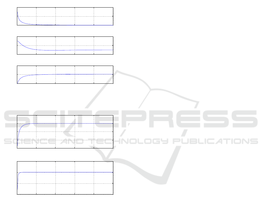
curve which ends up at the origin. Figure 4 shows

the convergence performance of the state variables. It

is shown that x

(t) converges to zero while x

(t) and

(t) each approach their desired value. The trajec-

tories are smooth and there is no overshoot or oscil-

lation. The whole process settles quickly within 0.5

seconds.

0 0.3 0.6 0.9 1.2 1.5

Figure 4: Convergence of the states.

0 0.3 0.6 0.9 1.2 1.5

−6

−4

−2

reaching control

0 0.3 0.6 0.9 1.2 1.5

−20

−10

equivalent control

Figure 5: Control signal u.

The variation of the control signal u during the pe-

riod is plotted in Figure 5.

As shown above, a good performance is achieved.

A higher order sliding behavior is shown.

5 CONCLUSIONS

In this paper, a new method of designing a higher or-

der sliding mode controller for a continuous nonlin-

ear dynamic system is reported. Retaining the advan-

tages of higher order sliding mode control, i.e. chat-

tering reduction, the complexity of nonlinear design is

greatly reduced with this method especially in reach-

ing control design. A ﬁeld-controlled DC motor is

given as an illustrative example to show the effective-

ness of this method.

REFERENCES

Vadim I. Utkin (1992). Sliding Modes in Control and Opti-

mization. Springer-Verlag New York, Inc.

Vadim I. Utkin (1977). Variable Structure Systems with

Sliding Modes. IEEE Transactions on Automatic Con-

trol, Volume AC-22, No. 2, April.

S. V. Emeryanov, S. K. Korovin, and A. Levant (1996).

Higher-order Sliding Modes in Control Systems.

Computational Mathematics and Modeling, Vol. 7,

No. 3.

A. Levant (2007). Principles of 2-sliding mode design. Au-

tomatica Vol. 43, pp. 576 – 586.

S. Laghrouche, F. Plestan, and A. Glumineau (2005). Multi-

variable practical higher order sliding mode control.

Proceedings of the 44th IEEE Conference on Decision

and Control, and the European Control Conference.

A.J. Koshkouei, K.J. Burnham and A.S.I. Zinober. Dynamic

sliding mode control design. IEE Proceedings online

no. 20055133.

I. Boiko, L. Fridman, and I. M. Castellanos (2004). Anal-

ysis of second-order sliding-mode algorithms in the

frequency domain. IEEE Transaction on Automatic

Control, Vol. 49, No. 6, pp. 946–950, Jun.

Vadim Utkin and Jingxin Shi(1996). Integral Sliding Mode

in Systems Operating under Uncertainty Conditions.

Proceedings of the 35th Conference on Decision and

Control, Kobe, Japan, December.

S. K. Spurgeon (2004). Temperature Control of Industrial

Process using a Variable Structure Design Philoso-

phy. Transactions of the Institute of Measurement and

Control

R. R. Bitmead, M. Gevers, and V. Wertz (1990). Adaptive

Optimal Control: The Thinking Man’s GPC. Engle-

wood Cliffs, NJ: Prentice-Hall.

Raymond, A. DeCarlo, Stanislaw H. Zak, Gregory P.

Matthews(1988). Variable Structure Control of Non-

linear Multivariable Systems: A Tutorial. Proceedings

of The IEEE, Vol. 76, No. 3, March.

Christopher Edwards and Sarah K. Spurgeon (1998). Slid-

ing Mode Control, Theory And Applications. CRC

Press, Taylor & Francis Group.

HIGHER ORDER SLIDING MODE CONTROL FOR CONTINUOUS TIME NONLINEAR SYSTEMS BASED ON

OPTIMAL CONTROL