
A NEW DECONVOLUTION METHOD BASED ON MAXIMUM
ENTROPY AND QUASI-MOMENT TRUNCATION TECHNIQUE
Monika Pinchas
Department of Electrical and Electronic Engineering, Ariel University Center of Samaria, Ariel 40700, Israel
Ben Zion Bobrovsky
Department of Electrical Engineering-Systems, Tel-Aviv University, Tel Aviv 69978, Israel
Keywords:
Blind equalization, Blind deconvolution, Non-linear adaptive filtering.
Abstract:
In this paper we present a new blind equalization method based on the quasi-moment truncation technique
and on the Maximum Entropy blind equalization method presented previously in the literature. In our new
proposed method, fewer moments of the source signal are needed to be known compared with the previously
presented technique. Simulation results show that our new proposed algorithm has better equalization perfor-
mance compared with Godard’s and Lazaro’s et al. algorithm.
1 INTRODUCTION
We consider a blind equalization problem in which
we observe the output of an unknown, possibly non-
minimum phase, linear system from which we want
to recover its input using an adjustable linear fil-
ter (equalizer). The problem of blind equalization
arises comprehensively in various applications such
as digital communications, seismic signal process-
ing, speech modeling and synthesis, ultrasonic non-
destructive evaluation, and image restoration (Feng
and Chi, 1999). Recently, a new blind equaliza-
tion algorithm was proposed (Pinchas and Bobrovsky,
2006) with improved equalization performance com-
pared with (Godard, 1980) and (Lazaro et al., 2005).
It is valid for the real and complex (where the real
and imaginary parts are independent) valued case.
This new blind equalization method (Pinchas and Bo-
brovsky, 2006) is based on the Maximum Entropy
technique and on some known moments of the source
signal. The problem arises when these moments or
part of them are unknown. In that case the blind
equalization method (Pinchas and Bobrovsky, 2006)
can not be used. Obviously, when using approximated
moments instead of the real ones, the equalization
performance might get worse and in some cases even
lead to unacceptable performance. The quasi-moment
truncation technique is related to the Hermite polyno-
mials where the high-order central moments are ap-
proximated in terms of lower order central moments
(Bover, 1978). Although the quasi-moment trunca-
tion technique (Bover, 1978) is well known in the
non-linear optimal filtering theory (Bover, 1978), it
is not yet been used in the field of blind equalization
combined with the Maximum Entropy technique. In
this paper we present a new blind equalization method
based on the quasi-moment truncation technique and
on the Maximum Entropy blind equalization method
(Pinchas and Bobrovsky, 2006). Fewer moments of
the source signal are needed to be known compared
with (Pinchas and Bobrovsky, 2006). Simulation re-
sults will show that our new proposed algorithm has
better equalization performance compared with Go-
dard’s (Godard, 1980) and Lazaro’s et al. (Lazaro
et al., 2005) algorithm. The paper is organized as fol-
lows: After having described the system under con-
sideration in Section II, we describe in Section III the
quasi-moment truncation technique which we use in
this paper for approximating the unknown source mo-
ments. In Section IV we present our simulation re-
sults and Section V is our conclusion.
2 SYSTEM DESCRIPTION
The system under consideration is illustrated in Fig.1,
where we make the following assumptions:
1. The input sequence x(n) consists of zero mean
210
Pinchas M. and Zion Bobrovsky B.
A NEW DECONVOLUTION METHOD BASED ON MAXIMUM ENTROPY AND QUASI-MOMENT TRUNCATION TECHNIQUE.
DOI: 10.5220/0002168902100213
In Proceedings of the 6th International Conference on Informatics in Control, Automation and Robotics (ICINCO 2009), page
ISBN: 978-989-674-001-6
Copyright
c
2009 by SCITEPRESS – Science and Technology Publications, Lda. All rights reserved

real or complex (where the real and imaginary part
of x(n) are independent) random variables with an
unknown even symmetric probability distribution.
2. The unknown channel h(n) is a possibly nonmin-
imum phase linear time-invariant filter in which the
transfer function has no “deep zeros”, namely, the
zeros lie sufficiently far from the unit circle.
3. The equalizer c(n) is a tap-delay line.
4. The noise w(n) is an additive Gaussian white
noise.
5. The function T[·] is a memoryless nonlinear
function. It satisfies the analyticity condition:
T(z
1
+ jz
2
) = T
1
(z
1
) + jT
2
(z
2
) where z
1
, z
2
, are
the real and imaginary part of the equalized output
respectively.
The transmitted sequence x(n) is transmitted
through the channel h(n) and is corrupted with noise
w(n). Therefore, the equalizer’s input sequence y(n)
may be written as:
y(n) = x(n) ∗h(n) + w(n) (1)
where ”∗” denotes the convolution operation. This
sequence (1) is then equalized with an equalizer c(n).
The equalizer’s output sequence z(n) may be written
as:
z(n) = x(n) ∗h(n) ∗c(n) + w(n) ∗c(n) =
x(n) + p(n) + ˜w(n)
(2)
where p(n) is the convolutional noise and ˜w(n) =
w(n) ∗c(n). In this paper, we consider the equalizer
proposed by (Pinchas and Bobrovsky, 2006) where
the equalizer’s taps are updated according to:
c
l
(n+ 1) = c
l
(n) −µWy
∗
(n−l) with
W = [(W
1
+W
2
) −z[n]]
W
1
= E
x
1
z
1
"
z
1
[n]E
x
1
z
1
h(z
1
)
2
i
n
#
W
2
= jE
x
2
z
2
"
z
2
[n]E
x
2
z
2
h(z
2
)
2
i
n
#
z
2
s
n
= (1−β)
z
2
s
n−1
+ β ·(z
s
)
2
n
(3)
where ()
∗
is the conjugate of (), µ is a positive step-
size parameter, l stands for the l-th tap of the equal-
izer, hi stands for the estimated expectation,
z
2
s
0
>
0 (s = 1, 2), β is a positive stepsize parameter and
E[x
s
/z
s
] (s = 1,2) is the conditional expectation de-
rived in (Pinchas and Bobrovsky, 2006) with the use
of the Maximum Entropy density approximationtech-
nique. This blind equalization algorithm (3) depends
on some known moments of the source signal through
the expression of the conditional expectation given in
(Pinchas and Bobrovsky, 2006). The problem arises
when we do not know these moments or we know
only a part of them. In that case we can not use the
algorithm. In the following we will show how we
solve this problem and still obtain satisfying equal-
ization performance compared with (Godard, 1980)
and (Lazaro et al., 2005).
3 MOMENT APPROXIMATION
In this section we use the quasi-moment truncation
technique (Bover, 1978) for approximating the un-
known source moments. In the following we con-
sider the real valued case. The quasi-moment trun-
cation technique is related to the Hermite polyno-
mials where the high-order central moments are ap-
proximated in terms of lower order central moments
(Bover, 1978). According to (Bover, 1978), one way
of achieving this is by expressing the probability den-
sity function f
x
(x) as an infinite series expansion in
which the coefficients are known in terms of central
moments. Then truncation approximations is done by
assuming that high-order coefficients in this expan-
sion are negligible. This would seem likely to oc-
cur when the basis for the expansion is an appropri-
ate set of orthogonal polynomials (Bover, 1978). A
natural choice of expansion basis is the Hermite poly-
nomials (Bover, 1978) which was used by Kuznetsov,
Stratonovich and Tikhonov (Kuznetsov et al., 1960)
who introduced the name “quasi-moment” for the ex-
pansion coefficients. Thus following (Bover, 1978),
the probability density function f
x
(x) is expressed as:
f
x
(x) =
1
√
2πσ
x
exp
−
x
2
2σ
2
x
∞
∑
L=0
b
L
L!
H
L
(x) (4)
where b
L
are the quasi-moments and H
L
(x) are the
Hermite polynomials defined by:
H
L
(x) = exp
x
2
2σ
2
x
−
d
dx
L
exp
−
x
2
2σ
2
x
(5)
According to (Bover, 1978), we may deduce quite
simple expressions for the quasi-moments in terms
of central moments by using the property, proved by
(Appel and Feriet, 1926), that the Hermite polyno-
mials are orthogonal with their adjoint polynomials,
with respect to a Gaussian weight function. By a
straight forward manipulation we may find that any
quasi-moment is equal to the expectation of the corre-
sponding adjoint Hermite polynomial (Bover, 1978),
namely:
b
L
=< G
L
(x) > where
G
L
(x) = exp
ex
2
σ
2
x
2
−
d
dex
L
exp
−
ex
2
σ
2
x
2
with ex =
x
σ
2
x
(6)
A NEW DECONVOLUTION METHOD BASED ON MAXIMUM ENTROPY AND QUASI-MOMENT TRUNCATION
TECHNIQUE
211

In the following is a list of the first six one-
dimensional quasi-moments calculated by (Bover,
1978):
b
0
= 1; b
1
= 0; b
2
= 0; b
3
=
x
3
b
4
=
x
4
−3
x
2
2
; b
5
=
x
5
−10
x
2
x
3
b
6
=
x
6
−15
x
2
x
4
+ 30
x
2
3
(7)
Now, assuming for instance that b
6
is negligible (b
6
=
0), an approximation for the six-th central moment in
terms of lower order central moments is obtained.
4 SIMULATION
In this section we investigate the equalization per-
formance by simulation where we use the residual
ISI (intersymbol interference) as a measure of per-
formance. Note that the ISI is often used as a mea-
sure of performance in equalizers’ applications. In
the following, we denote “MaxEnt” as the algorithm
described by (3) with the Lagrange multipliers given
in (Pinchas and Bobrovsky, 2006) where the required
source moments are known. The step-size parameters
for this method were denoted as µ and β and we sub-
stituted E[z
2
s
] = E[x
2
s
] for initialization. The equalizer
taps for Godard’s algorithm (Godard, 1980) were up-
dated according to:
c
l
(n+ 1) = c
l
(n)−
µ
G
|z(n)|
2
−
E
[
|x(n)|
4
]
E
[
|x(n)|
2
]
z(n)y
∗
(n−l)
(8)
where µ
G
is the step-size. The equalizer taps for al-
gorithm (Shalvi and Weinstein, 1990) were updated
according to:
c
′
i
(n+ 1) = c
′′
i
(n) + µ
SW
·sgnϒ(x)|z(n)|
2
z(n)·
y
∗
(n−i) where c
′′
i
(n) =
1
,
r
∑
i
|c
′
i
|
2
!
c
′
i
(9)
where c
′′
i
(n) is the vector of taps after iteration, c
′′
i
(0)
is some reasonable initial guess, µ
SW
is the step-size
and ϒ(x) = E
h
|x|
4
i
− 2E
2
h
|x|
2
i
−
E
x
2
2
is the
kurtosis associated to x. In the following, we denote
algorithm (Shalvi and Weinstein, 1990) as SW. The
equalizer taps for algorithm (Lazaro et al., 2005) were
updated according to:
c
l
(n+ 1) = c
l
(n)−
µ
par
1
N
sym
N
sym
∑
k=1
˜
K
′
σ
|z(n)|
2
−F (σ)|x
k
|
2
!!
·
z(n)y
∗
(n−l)
(10)
where µ
par
is the step-size,
˜
K
′
σ
(z) is the derivative of
˜
K
σ
(z) which is the Parzen window kernel of size σ
and F (σ) is the compensation factor that depends on
the kernel size. In (Lazaro et al., 2005) the Gaussian
kernel with standard deviation σ was used for
˜
K
σ
(z):
˜
K
σ
(z) =
1
√
2πσ
exp
−
z
2
2σ
2
. In the following, we de-
note algorithm (Lazaro et al., 2005) as SQD. We de-
note “MaxEntA” as the algorithm described by (3)
with the Lagrange multipliers given in (Pinchas and
Bobrovsky, 2006) where some of the required source
moments are approximated according to the quasi-
moment truncation technique (7). The step-size pa-
rameters for this method were denoted as µ
A
and β
A
and we substituted E[z
2
s
] = E[x
2
s
] for initialization un-
less otherwise stated. We used in our simulation a
16QAM source (a modulation using ± {1,3} levels
for in-phase and quadrature components). Two chan-
nels were considered. Channel1 (initial ISI = 0.44):
The channel parameters were determined according
to (Shalvi and Weinstein, 1990):
h
n
= {0 for n < 0; −0.4 for n = 0
0.84·0.4
n−1
for n > 0}
(11)
Channel2 (initial ISI = 1.402): The channel parame-
ters were taken according to (Lazaro et al., 2005):
h
n
= (0.2258,0.5161,0.6452,0.5161).
For Channel1 a 13-tap equalizer was used. For Chan-
nel2 we used an equalizer with 21 taps. In our sim-
ulation, the equalizers were initialized by setting the
center tap equal to one and all others to zero. The
step-size parameters µ, µ
A
, µ
G
, β, β
A
, µ
SW
, µ
par
were
chosen for fast convergence with low steady state ISI.
For the 16QAM source input propagating through
Channel2, the performance of Godard’s and SQD al-
gorithm were reproduced following (Lazaro et al.,
2005). For the 16QAM modulation source, two La-
grange multipliers (λ
2
, λ
4
) were used by the “Max-
Ent” and “MaxEntA” algorithm. For the “MaxEntA”
algorithm, m
6
was approximated according to the
quasi-moment truncation method while the other mo-
ments m
4
and m
2
were assumed to be known. Figure
2 shows the equalization performance of “MaxEnt”
and “MaxEntA” compared with (Lazaro et al., 2005)
and (Shalvi and Weinstein, 1990) for the 16QAM
source constellation propagating through channel1.
The performance is expressed in terms of residual ISI
as a function of iteration number. Figure 3 shows
the equalization performance of “MaxEntA” with and
without the use of initial samples for the initializa-
tion phase compared with (Lazaro et al., 2005) and
(Godard, 1980) for the 16QAM source constellation
propagating through channel2. According to the sim-
ulated results, our new proposed algorithm “Max-
EntA” has improved equalization performance com-
ICINCO 2009 - 6th International Conference on Informatics in Control, Automation and Robotics
212
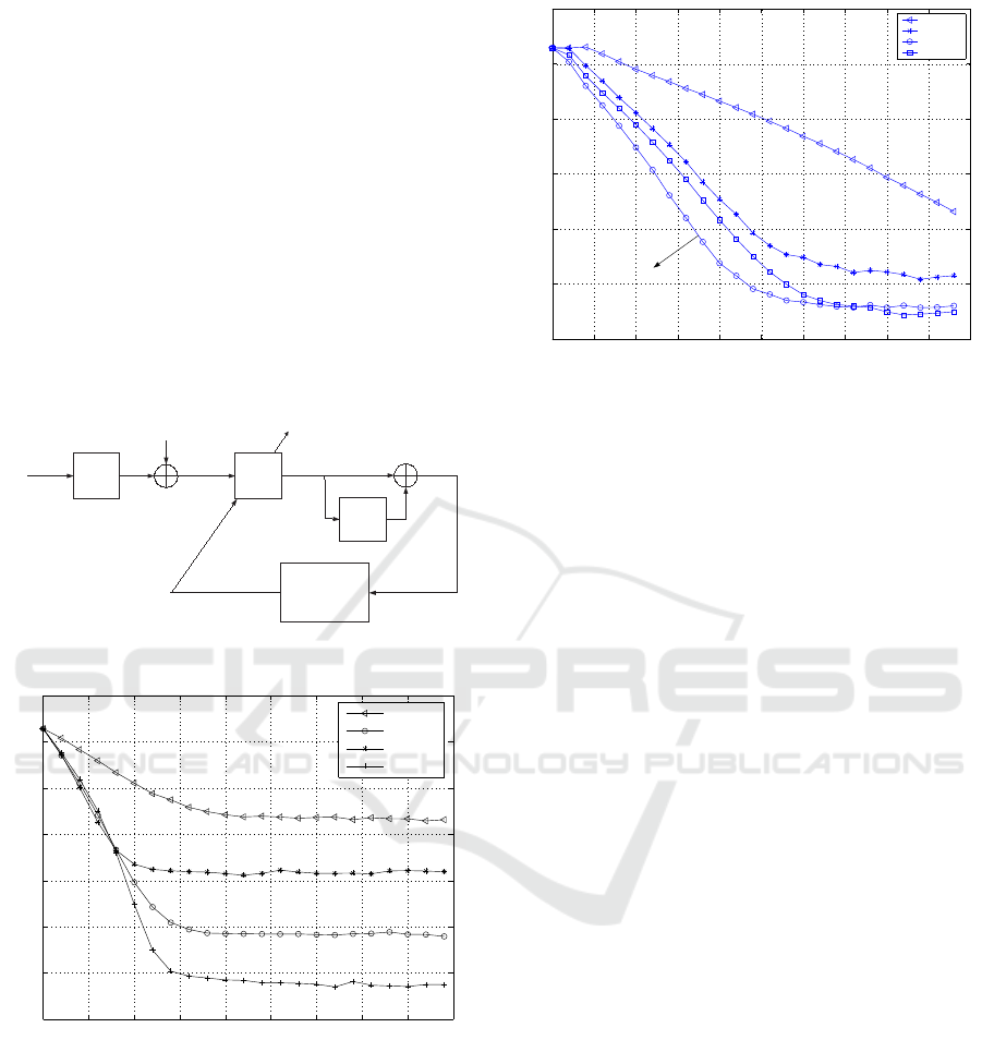
pared with (Godard, 1980), (Shalvi and Weinstein,
1990) and (Lazaro et al., 2005).
5 CONCLUSIONS
We have derivedin this paper a newblind equalization
method based on the quasi-moment truncation tech-
nique and on the Maximum Entropy blind equaliza-
tion method (Pinchas and Bobrovsky, 2006). In our
proposed algorithm, fewer moments of the source sig-
nal are needed to be known compared with (Pinchas
and Bobrovsky, 2006). Simulation results indicate
that the new proposed algorithm has improved equal-
ization performance compared with (Godard, 1980)
and (Lazaro et al., 2005).
h(n)
x(n)
c(n)
w(n)
y(n)
z(n)
Equalizer
T[ ]
d(n)
Adaptive Control
Algorithm
C(n+1)
+
+
+
-
Figure 1: Baseband communication system.
0 500 1000 1500 2000 2500 3000 3500 4000 4500
−35
−30
−25
−20
−15
−10
−5
0
Iteration Number
ISI [dB]
SW
MaxEntA
SQD
MaxEnt
Figure 2: Performance comparison between equalization al-
gorithms for a 16QAM source input going through chan-
nel1. The averaged results were obtained in 100 Monte
Carlo trials for a SNR of 30 (dB). The step-size parameters
were set to: µ
SW
= 2.5e-5, µ = 3e-4, β = 2e-4, µ
A
= 3.5e-4,
β
A
= 4e-4 and µ
par
= 2.5e-4. In addition we set F(σ) = 1,
σ = 15 and ε to 0.5, 0 for MaxEnt and MaxEntA respec-
tively.
0 1 2 3 4 5 6 7 8 9 10
x 10
4
−25
−20
−15
−10
−5
0
5
Iteration Number
ISI (dB)
Godard
SQD
MaxEntA
MaxEntA
initialized with 3000 samples
Figure 3: Performance comparison between equalization al-
gorithms for a 16QAM source input going through chan-
nel2. The averaged results were obtained in 50 Monte Carlo
trials for a SNR of 30 (dB). The step-size parameters were
set to: µ
A
= 2e-4, β
A
= 2e-6, µ
A
= 2.5e-4 for “o” , β
A
= 2e-
6 for “o”, µ
par
= 1e-4 and µ
G
= 1e-5. In addition we set
ε = 0.5, F(σ) = 1 and σ = 15.
REFERENCES
Appel, P. and Feriet, J. K. D. (1926). Fonctions hy-
pergeometriques et hyperspheriques. In polynomes
d’Hermite 367-369. Gauthier-Villars, Paris.
Bover, D. C. C. (1978). Moment equation methods for non-
linear stochastic systems. In Journal of Mathematical
Analysis and Applications 65 306-320.
Feng, C. and Chi, C. (1999). Performance of cumulant
based inverse filter for blind deconvolution. In IEEE
Transaction on Signal Processing 47 (7) 1922-1935.
IEEE.
Godard, D. (1980). Self recovering equalization and car-
rier tracking in two-dimentional data communication
system. In IEEE Transaction Communication 28 (11)
1867-1875. IEEE.
Kuznetsov, P. I., Stratonovich, R. L., and Tikhonov, V. I.
(1960). Quasi-moment functions in the theory of ran-
dom process. In Theor. Probability Appl. 5 80-97.
Lazaro, M., Santamaria, I., Erdogmus, D., Hild, K. E., Pan-
taleon, C., and Principe, J. C. (2005). Stochastic blind
equalization based on pdf fitting using parzen estima-
tor. In IEEE Transaction on Signal Processing 53 (2)
696-704. IEEE.
Pinchas, M. and Bobrovsky, B. Z. (2006). A maximum
entropy approach for blind deconvolution. In Signal
Processing Vol. 86, issue 10 2913-2931. Elsevier.
Shalvi, O. and Weinstein, E. (1990). New criteria for blind
deconvolution of nonminimum phase systems (chan-
nels). In IEEE Trans. Information Theory 36 (2), 312-
321.
A NEW DECONVOLUTION METHOD BASED ON MAXIMUM ENTROPY AND QUASI-MOMENT TRUNCATION
TECHNIQUE
213
