INDUCED ℓ

∞

− OPTIMAL GAIN-SCHEDULED FILTERING OF

AKAGI-SUGENO FUZZY SYSTEMS

Isaac Yaesh

Control Department, IMI Advanced Systems Div., P.O.B. 1044/77, Ramat–Hasharon, 47100, Israel

Uri Shaked

School of Electrical Engineering, Tel Aviv University, Tel Aviv, 69978, Israel

Keywords:

Takagi-Sugeno fuzzy systems, Polytopic uncertainties, H

∞

-optimization, ℓ

∞

-optimization, S -procedure, Lin-

ear matrix inequalities.

Abstract:

The problem of designing gain-scheduled ﬁlters with guaranteed induced ℓ

∞

norm for the estimation of the

state-vector of ﬁnite dimensional discrete-time parameter-dependent Takagi-Sugeno Fuzzy Systems systems

is considered. The design process applies a lemma which was recently derived by the authors of this paper,

characterizing the induced ℓ

∞

norm by Linear Matrix Inequalities. The suggested ﬁlter has been successfully

applied to a guidance motivated estimation problem, where it has been compared to an Extended Kalman

Filter.

1 INTRODUCTION

The theory of optimal design of estimators for linear

discrete-time systems in a state-space formulation has

been ﬁrst established in (Kalman, 1960). The original

problem formulation assumed Gaussian white noise

models for both the measurement noise and the ex-

ogenous driving process. For this case, the results

of (Kalman, 1960) provided the Minimum-Mean-

Square Estimator (MMSE). The Kalman ﬁlter has

found since then many applications (see e.g. (Soren-

son, 1985) and the references therein). Following the

introduction of H

∞

control theory in (Zames, 1981),

a method for designing discrete-time H

∞

optimal es-

timators within a deterministic framework has been

developedin (Yaesh and Shaked, 1991), where the ex-

ogenous signals are of ﬁnite energy. The case where

the driving signal is of ﬁnite energy (e.g. piecewise

constant for a ﬁnite time) ,whereas the measurement

noise is white has been recently considered in (Yaesh

and Shaked, 2006). However, in some cases the min-

imization of the maximum absolute value of the es-

timation error (namely the ℓ

∞

−norm) rather than the

error energy is required where the exogenous signals

are also of ﬁnite ℓ

∞

−norm. In such cases, an induced

ℓ

∞

−norm is obtained which is often referred to as an

ℓ

problem due to the fact that the induced-ℓ

∞

−norm

for a linear system is just the ℓ

-norm of its impulse

response and an upper-bound on the ℓ

-norm of its

transfer function (see (Dahleh and Pearson, 1987)).

In the present paper, the problem of discrete-

time optimal state-estimation in the minimum in-

duced ℓ

∞

−norm sense is considered for a class of

Takagi-Sugeno fuzzy systems. The plant model for

the systems considered, is described by a collection

of ’sample’ ﬁnite-dimensional linear-time-invariant

plants which possess the same structure but differ

in their parameters. All possible plant models are

then assumed to be convex combinations of these spe-

ciﬁc plant models (namely a polytopic system where

the ’sample’ plant models are denoted as its vertices

(Boyd et al., 1994)). The solution of the estima-

tion problem is characterized by LMIs (Linear Ma-

trix Inequalities) based on the quadratic stability as-

sumption. We note that more recent developments of

(Geromel et al., 2000) include gain scheduled ﬁlter

synthesis for the cases of linear (Tuan et al., 2001)

and nonlinear (Hoang et al., 2003) dependence on the

parameterswith parameter dependentLyapunovfunc-

tions. We also note that in (Salcedo and Martinez,

2008) related results appear where the continuous-

time fuzzy output feedback and ﬁltering were con-

sidered in parallel to the discrete-time results of the

present paper.

The paper is organized as follows. In Section 2,

the problem is formulated and a key lemma character-

Yaesh I. and Shaked U.

INDUCED â

D ¸Sâ

d â

LŠ OPTIMAL GAIN-SCHEDULED FILTERING OF TAKAGI-SUGENO FUZZY SYSTEMS.

DOI: 10.5220/0002169500670073

In Proceedings of the 6th International Conference on Informatics in Control, Automation and Robotics (ICINCO 2009), page

ISBN: 978-989-674-001-6

izing the induced ℓ

∞

−norm in terms of LMIs is pre-

sented. In Section 3 the ﬁlter design inequalities are

obtained. Section 4 considers a numerical example

dealing with a robust gain scheduled tracking prob-

lem. Finally, Section 5 brings some concluding re-

marks.

Notation: Throughout the note the superscript

‘T’ stands for matrix transposition, R

denotes the

n dimensional Euclidean space, R

n×m

is the set of

all n ×m real matrices, and the notation P > 0, for

P ∈R

n×n

means that P is symmetric and positive def-

inite. The space of square summable functions over

[0 ∞] is denoted by l

[0 ∞], and ||.||

stands for the

standard l

-norm,||u||

= (Σ

∞

k=0

)

1/2

. We also use

||.||

∞

for the l

∞

-norm namely, ||u||

∞

= sup

The convex hull of a and b is denoted by C o{a, b},

is the unit matrix of order n, and 0

n,m

is the n ×m

zero matrix and I

m,n

is a version of I

with last n−m

rows omitted.

2 PROBLEM FORMULATION

AND PRELIMINARIES

We consider the following linear system:

x(k+ 1) = A(k)x(k) + Bw(k), x(0) = x

y(k) = C(k)x(k) + Dw(k)

z(k) = L(k)x(k)

(1)

where x ∈ R

is the system states, y ∈R

is the mea-

surement, w ∈ R

includes the driving process and

the measurement noise signals and it is assumed to

have bounded ℓ

∞

−norm. The sequence z ∈ R

is the

state combination to be estimated and A, B, C, D and

L are matrices of the appropriate dimensions.

We assume that the system parameters lie within

the following polytope

Ω :=



A B C D L



(2)

which is described by its vertices. That is, for

Ω





(3)

we have

Ω = C o{Ω

,Ω

,...,Ω

} (4)

where N is the number of vertices. In other words:

Ω =

∑

i=1

Ω

∑

i=1

= 1 , f

≥ 0. (

Assuming that f

are exactly known, the above sys-

tem is just a Tagaki-Sugeno fuzzy system. To see this,

one may introduce new parameters s

(t),i = 1, 2,..., p

(so called premise variables, see (Tanaka and Wang,

2001)) possibly depending on the state-vector x(t),

external disturbances and/or time (Tanaka and Wang,

2001) and rewrite (1) as :

IF s

is M

and s

is M

and ... s

is M

THEN

x(k+ 1) = A

(k)x(k) + B

w(k), x(0) = x

y(k) = C

(k)x(k) + D

w(k)

z(k) = L

(k)x(k)

i = 1, 2,..., N

(6)

where M

is the fuzzy set and N is the

number of model rules. Deﬁning s(t) =

col{s

(t),s

(t),...,s

(t)},

(s(t)) = Π

j= 1

(t))

and

(s(t)) =

(t)

i=1

(s(t))

we readily get the representation of (1). We, there-

fore, assume indeed that the p premise scalar vari-

ables s

(t),i = 1,2,..., p, and, consequently f

are ex-

actly known and consider the following ﬁlter:

ˆx(k+ 1) = Aˆx(k) + K(k)(y−Cˆx), ˆz(k) = Lˆx(k)

(7)

where the ﬁlter gain is given by the following:

K =

∑

i=1

(8)

and where A =

∑

i=1

and L =

∑

i=1

. We will dif-

ferently treat, in the sequel, the case where C is con-

stant and the case where C =

∑

i=1

Our aim is to ﬁnd the ﬁlter parameters K

so that

the following induced ℓ

∞

−norm condition is satisﬁed.

sup

w∈ℓ

∞

||z− ˆz||

∞

/||w||

∞

< γ (9)

To solve this problem we will ﬁrst deﬁne another

polytopic system :

Ω :=





(10)

which is described by the vertices:

Ω





, i = 1,...,N (11)

The system of (10)-(11) will represent, in the sequel,

the dynamics of the estimation error for the system

(1). The following technical lemma will be needed

in order to provide convex characterization of the in-

duced ℓ

∞

− norm of the estimation error system:

Lemma 1. The system

¯x(k+ 1) =

A(k) ¯x(k) +

Bw(k), x(0) = x

z(k) =

C(k) ¯x(k) +

D ¯w(k)

(12)

satisﬁes

sup

w∈ℓ

∞

||z||

∞

/||w||

∞

< γ (13)

ICINCO 2009 - 6th International Conference on Informatics in Control, Automation and Robotics

if the following matrix inequalities are satisﬁed for

i = 1,2,

...,N:



+ λP−P

−µI +



< 0 (14)

and





λP 0

0 (γ−µ)I

γI





> 0 (15)

so that P > 0, µ > 0 and λ < 1.

The proof of this lemma is given in (Shaked and

Yaesh, 2007) and is also provided, for the sake of

completeness, in Appendix A.

Remark. Note that (14) can be written, using

Schur complements ((Boyd et al., 1994)), as follows:





P−λP 0

0 µI





> 0 (16)

or equivalently as





P−λP 0

0 µI

−1





> 0 (17)

The fact that the inequality (16) is afﬁne in

and

will be utilized in the sequel to obtain convex charac-

terization (i.e. in LMI form) of the ﬁlter parameters

3 GAIN SCHEDULED FILTERING

Deﬁning the state estimation error to be:

e(k) = x(k) − ˆx(k) (18)

we readily have for the case where f

are available for

the estimation process, that

e(k+ 1) = (A−K(k)C)e(k) + (B−K(k)D)w(k)

(19)

and

z(k) − ˆz(k) = Le(k) (20)

We substitute

= A

−K

= B

−K

D and

C = L

in (14) and (15) where we restrict our attention

to the case where C and D are not vertex dependent

(i.e. C

= C,D

= D,i = 1,2, ...,N). In this case, we

deﬁne Y

= PK

and readily obtain from (16) and (15)

that





P−λP 0 A

P−C

0 µI B

P−D

−Y

C PB

−Y

D P





> 0

(21)

and





λP 0 L

0 (γ−µ)I 0

0 γI





> 0, λ < 1 (22)

We, therefore, obtain the following result:

Theorem 1. Consider the estimator of (12) for the

system of (1) with C

= C, D

= D,i = 1, 2,..., N. The

estimation error satisﬁes (9) if (21) and (22) are satis-

ﬁed for i = 1, 2,..., N so that P > 0, µ > 0 and λ < 1.

We next address the problem where C and D are

vertex dependent. To this end we consider a version

of Lemma 1 which can be written in terms of Ω rather

than Ω

, namely we replace (16) and (14) by:





P−λP 0

0 µI

A P

B P





> 0 (23)

and





λP 0

0 (γ−µ)I

D γI





> 0 (24)

and substitute

A =

∑

i, j=1

− K

) f

∑

i, j=1

−K

) f

and

C =

∑

i=1

. We obtain

deﬁning Y

= PK

∑

i, j=1

> 0 (

25)

where





P−λP 0 A

P−C

0 µI B

P−D

−Y





(26)

and

∑

i=1





λP 0 L

0 (γ−µ)I 0

0 γI





> 0 (

27)

Since, however (see (Tanaka and Wang, 2001))

equation (25) can be also written as

∑

i, j=1

∑

i=1

+ 2

∑

i=1

∑

i< j

+ G

(

28)

Deﬁning a simple transformation of the convex co-

ordinates f

so that for k = 1,2,...,N we set h

= f

where as the remaining h

for k = N+1,N+2,...,N+

N(N−1)

re deﬁned by h

= 2f

, j = 1,2...,N,i < j.

Since obviously

∑

N+

N(N−1)

k=1

= 1

where h

≥ 0 they

can serve as convex coordinates. We, therefore, deﬁne

the following LMIs inspired by (Tanaka and Wang,

2001),

> 0,i = 1, 2,...N and G

+ G

> 0,i < j (29)

INDUCED - OPTIMAL GAIN-SCHEDULED FILTERING OF TAKAGI-SUGENO FUZZY SYSTEMS

and obtain the following result:

Theorem 2. Consider the estimator (12) for the

system (1). The estimation error satisﬁes (9) if (29)

and (22) for i = 1,2,...,N are satisﬁed so that P > 0,

µ > 0 and λ < 1.

The solution offered above, for the case where C

and D are uncertain and are known to reside in a given

polytope, seeks a single matrix P that solves the LMIs

for

N(N+1)

vertices, instead of the N vertices that were

solved for in the case of known C and D. A solu-

tion for such large number of vertices by a single P

entails a signiﬁcant overdesign. Even the relaxation

offered by e.g. (Shaked, 2003) to reduce the overde-

sign by allowing different P

,i = 1,2,...,

N(N+1)

for

the

N(N+1)

vertices still suffers from a considerable

conservatism. Moreover, the computational complex-

ity of the solution also rapidly increases as a function

of the number of vertices.

In many cases,C resides in some uncertainty poly-

tope, while D is ﬁxed and known. In such a case, an

alternative way to deal with the problem is to deﬁne

ξ(k) = col{x(k), y(k)} and ˜w(k) = col{w(k), w(k +

1)}so that the augmented system becomes:

ξ(k+ 1) =

A(k)x(k) +

B ˜w(k)

y(k) =

C(k)ξ(k) +

D ˜w(k)

z(k) =

L(k)ξ(k)

where



A 0

CA 0





B 0

CB D





0 I





L 0



, and

D =



D 0



(30)

In (30) the uncertainties appear in

A and

B only and,

therefore, Theorem 1 above may be invoked. We,

therefore, obtain the following result which offers

reduced conservatism with respect the correspond-

ing continuous-time results of (Salcedo and Martinez,

2008):

Theorem 3. Consider the estimator of (12) for the

system of (1) for D

= D, i = 1,2,...,N. The estima-

tion error satisﬁes (9) with γ replaced by

√

2γ if (21)

and (22) are satisﬁed for i = 1,2, ...,N so that P > 0,

µ > 0 and λ < 1 with A,B,C,L replaced by

of (30).

4 EXAMPLE

We consider the dynamic model of guidance in a

plane:

˜x = νcos(

ψ) + w

˜y = νsin(

ψ) + w

ψ =

φ = −φ/τ+ u/τ

(31)

where ˜x and ˜y are the ﬁrst two coordinates of a ﬂight

vehicle cruising in a constant altitude, in a local level

north-east-down system,

ψ is the vehicle body an-

gle with respect to the north (i.e. azimuth angle)

and φ is the vehicle’s roll angle assumed to be gov-

erned by a ﬁrst-order low-pass ﬁlter dynamics hav-

ing a time-constant of τ seconds, driven by the roll-

angle command u. The wind velocities at the north

and east directions respectively are denoted by w

and

whereas ν is the true-air-speed. Our aim is to ﬁlter

the noisy measurements of ˜x, ˜y and φ and to estimate

ψ. Deﬁning,

x = col{˜x, ˜y,vsin(

ψ),vcos(

ψ),φ}

the measurements vector which consists of noisy

measurements of the position components ˜x and ˜y and

the roll angle φ is given by

y = Cx+ R

1/2

where v is the measurement noise which is taken in

the simulations in the sequel as a 3-vector of zero-

mean unity variance white noise sequences but for all

practical purposes is assumed to be v ∈ ℓ

∞

. The noise

level is set by

R = diag{25, 25,0.1}

and the measurement matrix is

C =





1 0 0 0 0

0 1 0 0 0

0 0 0 0 1





Note that

˙x

= x

˙x

= x

˙x

= x

˙x

= −x

˙x

= −x

/τ+ u/τ

(32)

namely we have a bilinear system rather than a lin-

ear one. Following (Tanaka and Wang, 2001) with

a series of simple manipulations, this system can be

represented as a Takagi-Sugeno fuzzy system, namely

as a convex combination of linear systems where the

convex coordinates are online measured. To achieve

such a representation we recall that x

= φ is mea-

sured on line, and deﬁne s

= x

while neglecting

the small enough noise in measuring φ. The valid-

ity of the latter assumption will be veriﬁed in the se-

quel by the estimation quality we will obtain. Assum-

ing x

∈ [−φ

max

,φ

max

] we deﬁne f

−s

1,min

1,max

−s

1,min

ICINCO 2009 - 6th International Conference on Informatics in Control, Automation and Robotics

+φ

2φ

, f

= 1− f

, α

= φ

max

and α

= −φ

max

. We

readily see that s

= φ

max

−φ

max

:= α

+ α

We note then that the system is then governed by

ξ = A

(ξ)ξ+ B

w where ξ = col{x

}and







0 0 0 1 0

0 0 1 0 0

0 0 0 s

0 0 −s

0 0

0 0 0 0 −1/τ







Therefore, A

= A

c,1

+ A

c,2

where A

c,1

is ob-

tained from A

by replacing s

by α

and A

c,2

is sim-

ilarly obtained from A

by replacing s

by α

. We

also deﬁne w = col{w

,ν

} and complete

the remaining matrices needed for the representation

of our problem (1)-(3) by applying a zero-order-hold

discrete-time equivalent of our continuous-time sys-

tem, where we have chosen a sampling time of h =

0.02. Due to the small enough h we have chosen, we

have e

= I + Ah+ O(h

) and we, therefore, readily

obtain that the system is governed by (1) and (3)-(5)

where A = A

+ A

+ O(h

) where







1.0000 −0.0002 0.0200 0

0 1.0000 0.0200 0.0002 0

0 0 0.9998 0.0209 0

0 0 −0.0209 0.9998 0

0 0 0 0 0.9231













1.0000 0 0.0002 0.0200 0

0 1.0000 0.0200 −0.0002 0

0 0 0.9998 −0.0209 0

0 0 0.0209 0.9998 0

0 0 0 0 0.9231







= B

= B =







0.2000 0 0 0 0

0 0.2000 0 0 0

0 0 0 0 0







and

= D

= D =





0 0 2.2361 0 0

0 0 0 2.2361 0

0 0 0 0 0.1000





We note at his point that, in order to mini-

mize the design conservatism stemming from the

quadratic stability assumption, we applied a pa-

rameter dependent Lyapunov function (Boyd et al.,

1994), max(x

x,x

x). Minimization of γ sub-

ject the the LMis that are obtained with this func-

tion to replace (21) and (22) (see Appendix B), us-

ing fminsearch.m from the optimization toolbox of

MATLAB

and (Lagarias et al., 1998) to search

, i = 1,2,3,4, ρ

, ρ2

, θ

and θ

, has resulted in

γ = γ

= 10.2732 and λ = 2.41×10

−7

. The follow-

ing gain matrices K

and K

have been obtained for

γ = γ

were obtained:







0.7574 −0.0007 0.0000

−0.0018 0.7593 0.0000

0.0000 0.0000 0.0000

0.0000 −0.0000 0.0000

−0.0000 −0.0000 0.0003













0.7558 −0.0024 0.0000

−0.0021 0.7613 −0.0000

−0.0000 0.0000 −0.0000

0.0000 0.0000 0.0000

−0.0000 0.0000 0.0003







This ℓ

∞

ﬁlter will be compared to an Extended

Kalman Filter (EKF, see (Jazwinsky, 1970)) based on

the nonlinear model of (31). Note that higher com-

plexity ﬁlters such as the particle ﬁlter (e.g. (Osh-

man and Carmi, 2006) are out the scope of the

present paper. For the simulations we take ν =

100m/s and try to control the vehicle to follow a

constant command at y = 5m, in spite of a wind

step at w

of 10m/s. The estimation results are

used to control the vehicle, using the simple law

u = −



0.0200 4.0000



ˆy−5



where all

components of the initial state-vector are taken as

zero, besides y

= 20m. The EKF and the ℓ

∞

esti-

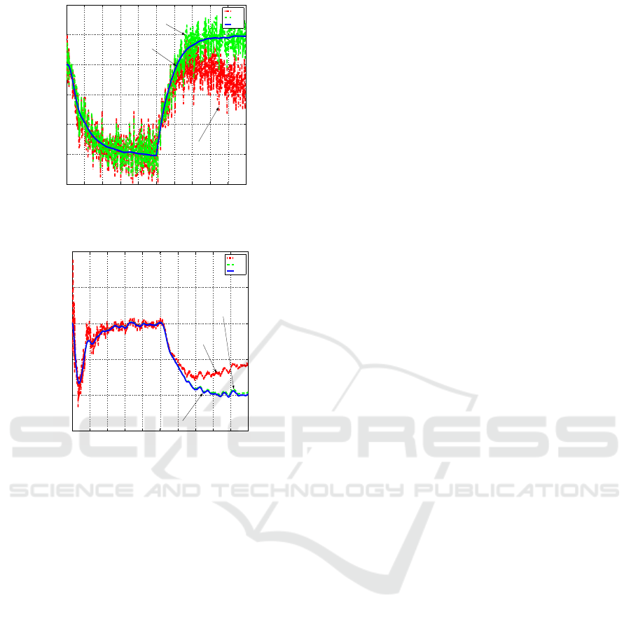
mated ˜x− ˜y trajectory results are compared in Fig. 1

to the true trajectory. One can notice the bias in the

EKF estimate. In Fig. 2, the true

ψ and the estimated

values for

ψ that are obtained by using the EKF and

the ℓ

∞

ﬁlter are depicted. We clearly see in this ﬁgure

that the ℓ

∞

ﬁlter outperforms the EKF which assumes

a white noise w

but leads to a bias when w

has a

bias. In contrast, the

ψ estimate of the ℓ

∞

ﬁlter is

barely separable from the true values. Moreover, the

ℓ

∞

ﬁlter does not require the on-line numerical solu-

tion of a Riccati equation of order 4 and the gains are

obtained there by a simple convex interpolation on K

and K

. The fact that K

and K

are close to each

other is somewhat surprising. Our experience shows

that for a larger γ (i.e. suboptimal values), a larger

||K

−K

|| is obtained.

5 CONCLUSIONS

The problem of designing robust gain-scheduled ﬁl-

ters with guaranteed induced ℓ

∞

−norm has been con-

sidered. The solution has been derived using a re-

cently developed bounded-real-lemma like condition

for bounding the induced ℓ

∞

norm of a system. This

result has been applied to derive the robust induced

ℓ

∞

−ﬁlter (or equivalently robust ℓ

ﬁlter) in terms of

LMIs. These LMIs have been applied to a guidance

motivated estimation example. In this example, the

INDUCED - OPTIMAL GAIN-SCHEDULED FILTERING OF TAKAGI-SUGENO FUZZY SYSTEMS

0 200 400 600 800 1000 1200 1400 1600 1800 2000

x [m]

y [m]

EKF

∞

True

∞

True

EKF

Figure 1: True, Extended Kalman Filter and ℓ

∞

-Filter Esti-

mated Trajectories - ˜x(t) versus ˜y(t).

0 2 4 6 8 10 12 14 16 18 20

−0.15

−0.1

−0.05

0.05

0.1

Time [sec]

EKF

∞

True

EKF

∞

True

Figure 2: True, Extended Kalman Filter and ℓ

∞

-Filter Esti-

mated Azimuth Angle -

ψ versus t.

superiority of the induced ℓ

∞

ﬁlter over the Extended

Kalman Filter has been demonstrated, both in terms

of performance and simplicity of implementation.

REFERENCES

Abedor, J., Nagpal, K., and Poolla, K. (1996). A linear

matrix inequality approach to peak-to-peak gain min-

imization. International J. of Robust and Nonlinear

Control, 6:899–927.

Boyd, S., El-Ghaoui, L., Feron, L., and Balakrishnan, V.

(1994). Linear matrix inequalities in system and con-

trol theory. SIAM.

Dahleh, M. A. and Pearson, J. (1987). ℓ

-optimal feedback

controllers for mimo discrete-time systems. IEEE

Trans. on Automat. Contr., AC-32:314–322.

Geromel, J., Bernussou, J., Garcia, G., and de Oliviera, M.

(2000). h

and h

∞

robust ﬁltering for discrete-time

linear systems. SIAM Journal of Control and Opti-

mization, 38:1353–1368.

Hoang, N., Tuan, H., Apkarian, P., and Hosoe, S. (2003).

Robust ﬁltering for uncertain nonlinearly parame-

terized plants. IEEE Trans. on Signal Processing,

51:1806–1815.

Jazwinsky, A. H. (1970). Stochastic Processes and Filtering

Theory. Academic Press, New-York.

Kalman, R. (1960). A new approach to linear ﬁltering and

prediction problems. Transactions ASME, Journal of

Basic Engineering, 82d:35–45.

Lagarias, J., Reeds, J. A., Wright, M. H., and Wright, P. E.

(1998). Convergence properties of the nelder-mead

simplex method in low dimensions. SIAM Journal of

Optimization, 9:112–147.

Oshman, Y. and Carmi, A. (2006). Attitude estimation

from vector obsevations usinga genetic algorithm-

embedded quaternion particle ﬁlter. Journal of Guid-

ance, Control and Dyanmics, 29:879–891.

Salcedo, J. V. and Martinez, M. (2008). Bibo stabilization of

takagi-sugeno fuzzy systems under persistent pertur-

bations using fuzzy output feedback controllers. IET

Control Theory and Applications, 2:513–523.

Shaked, U. (2003). An lpd approach to robust h

and h

∞

static output-feedback design. IEEE Trans. on Au-

tomat. Contr., 48:866–872.

Shaked, U. and Yaesh, I. (2007). Robust servo synthesis

by minimization of induced ℓ

and ℓ

∞

norms. In ISIE

2007, Vigo, Spain.

Sorenson, H. (1985). Kalman Filtering : Theory and Appli-

cation. IEEE Press.

Tanaka, K. and Wang, H. (2001). Fuzzy Control Systems

Design and Analysis - A Linear Matrix Inequality Ap-

proach. John Wiley and Sons, Inc.

Tuan, H. D., Apkarian, P., and Nguyen, T. Q. (2001). Ro-

bust and reduced-order ﬁltering: new lmi-based char-

acterizations and methods. IEEE Trans. on Signal

Processing, 40:2975–2984.

Yaesh, I. and Shaked, U. (1991). A transfer function ap-

proach to the problems of discrete-time systems h

∞

optimal control and ﬁltering. IEEE Trans. on Automat.

Contr., 36:1264–1271.

Yaesh, I. and Shaked, U. (2006). Discrete-time min-max

tracking. IEEE Trans. Aerospace and Elect. Systems,

42:540–547.

Zames, G. (1981). Feedback and optimal sensitivity : model

reference transformations, multiplicative seminorms

and approximate inverses. IEEE Trans. on Automat.

Contr., AC-26:301–320.

APPENDIX A - PROOF OF

LEMMA 1

Consider the system

k+1

, z

and deﬁne, following (Abedor et al., 1996),

= x

k+1

−x

+ λx

−µw

Namely,

=(x

)P(

)−x

+λx

−µw

ICINCO 2009 - 6th International Conference on Informatics in Control, Automation and Robotics

Collecting terms we have

= x

(

A+ λP−P)x

+ x

(

B)w

(

A)x

+ w

(−µ

I +

B)w

Therefore, (14) guarantees ξ

< 0 for all w

and x

Deﬁning ζ

= x

and assuming x

= 0 and

< 1 we have that ζ

k+1

−ζ

+ λζ

−µw

< 0.

Namely, ζ

where

k+1

= (1 −λ)

+ µw

However, using ρ := 1−λ we have

k−1

∑

j= 0

k−j−1

µw

= ρ

k−1

∑

j= 0

(ρ

−1

)

µw

<ρ

k−1

(1−ρ

−1

)

1−ρ

−1

µ= µ

1−ρ

. A.1

rom (15) we have using Schur complements that

](



λP 0

0 (γ−µ)I



−γ

−1









)





> 0

Namely,

< γ[(γ−µ)w

+λx

] < γ[(γ−µ)+λ

] A.2

Substituting A.1 we readily see that

< γ[(γ−µ)+(1−ρ)µ

1−ρ

]

= γ[γ−µ+µ−µρ

Since 0 < ρ < 1 we obtain that

< γ[γ −µ+ µ] = γ

APPENDIX B - PARAMETER

DEPENDENT RESULTS

In order to reduce conservatism, we replace in the

proof of Lemma 1 in Appendix A, the parameter-

independent Lyapunov function V(x, P) = x

the parameter-dependent Lyapunov function ((Boyd

et al., 1994)) V(x,P

) = max(x

). To

ensure V(x

) > 0 we have to satisfy x

> 0

whenever x

> x

and x

> 0 whenever

< x

. Applying the S-procedure (Boyd

et al., 1994) we readily obtain that a sufﬁcient condi-

tion or these requirements to hold, is the existence of

constants ρ

> 0 and ρ

> 0 so that

−ρ

−P

) > 0 and P

−ρ

−P

) > 0.

We also require that if x

x > x

then

{1},

:= x

(

A+ λP

−P

+ x

(

B)w

(

A)x

+ w

(−µI +

B)w

< 0,

and if x

x > x

then

{2},

:= x

(

A+ λP

−P

+ x

(

B)w

(

A)x

+ w

(−µI +

B)w

< 0.

Since these conditions are required to be satisﬁed

throughout the polytope, we readily obtain, using

again the S-procedure, that in addition to the con-

stant λ > 0, the existence of six additional constants

> 0, i = 1,2,3, 4, θ

> 0, θ

> 0 establishes a suf-

ﬁcient condition for the above inequalities to hold, if

−ξ

{1},

−λ

−P

) > 0, i = 1, 2

and

−ξ

{1},

−λ

−P

) > 0,i = 1, 2.

Following the lines of proof of Theorem 1 above, we

readily obtain the following LMIs for i = 1,2 to re-

place (21) and (22):





−λP− λ

−P

) 0 A

−C

0 µI B

−D

−Y

C P

−Y

D P





>0,





λP

−θ

−P

) 0 L

0 (γ−µ)I 0

0 γI





> 0, λ < 1

and





−λP− λ

i+2

−P

) 0 A

−C

0 µI B

−D

−Y

C P

−Y

D P





>0,





λP

−θ

−P

) 0 L

0 (γ−µ)I 0

0 γI





> 0, λ < 1.

We note that we have also replaced (A.2) with:

< γ[(γ−µ)w

+λ×max(x

)].

Namely, if x

x > x

x we require

< γ[(γ−µ)w

+ λx

x],

whereas if x

x > x

x we require

< γ[(γ−µ)w

+ λx

x].

Using again the S -Procedure with additional tuning

constants θ

> 0 and θ

> 0, which add up to the pre-

viously introduced 7 tuning constants ρ

> 0, ρ

> 0,

λ > 0 and λ

> 0,i = 1, 2,3,4 the above results are

obtained. Note that a similar approach can be applied

also on the continuous-time results of (Salcedo and

Martinez, 2008) to reduce conservatism.

INDUCED - OPTIMAL GAIN-SCHEDULED FILTERING OF TAKAGI-SUGENO FUZZY SYSTEMS