
A NEW METHOD OF TUNING THREE TERM
CONTROLLERS FOR DEAD-TIME PROCESSES
WITH A NEGATIVE/POSITIVE ZERO
K. G. Arvanitis, G. D. Pasgianos
Department of Natural Resources Management and Agricultural Engineering
Agricultural University of Athens, 75 Iera Odos Str., 11855, Athens, Greece
A. K. Boglou
Technology Education Institute of Kavala, 65404, Agios Loukas, Kavala, Greece
N. K. Bekiaris-Liberis
Department of Mechanical and Aerospace Engineering, University of California
San Diego, La Jolla, CA 92093-0411, U.S.A.
Keywords: Process Control, PID Control, Dead-Time Processes, Process Zeros.
Abstract: The use of the Pseudo-Derivative Feedback (PDF) structure in the control of stable or unstable dead-time
processes with a negative or a positive zero is investigated. A simple direct synthesis method for tuning the
PDF controller is presented. Moreover, a modification of the proposed method, which ensures its
applicability in the case of large overshoot response processes with dead time, is also presented. The PDF
control structure and the proposed tuning method ensure smooth closed-loop response to set-point changes,
fast regulatory control and sufficient robustness against parametric uncertainty. Simulation results show
that, in most cases, the proposed method is as efficient as the best of the most recent PID controller tuning
methods for dead-time processes with negative/positive zeros, while its simplicity in deriving the controller
settings is a plus point over existing PID controller tuning formulae.
1 INTRODUCTION
In the process industry, stable second order dead-
time models as well as second order dead-time
models with one right-half-plane pole are frequently
used to adequately describe numerous processes for
the purpose of designing controllers. However, these
types of process models are inadequate in the case
where a process controlled variable encounters two
(or more) competing dynamic effects with different
time constants from the same manipulated variable
(Waller and Nygardas, 1975). This composite
dynamics results to a process behaviour that exhibits
an inverse response or a large overshoot response.
Inverse response or large overshoot response is port-
rayed by the presence of one (or an odd number of)
positive or negative zeros, respectively, in the
process models, and they can cause, together with
the process dead-times, serious problems in
designing and tuning simple controllers for the pro-
cess under consideration.
Inverse response second order dead-time process
models (SODT-IR) are used to represent the
dynamics of several chemical processes (like level
control loops in distillation columns and temperature
control loops in chemical reactors), as well as the
dynamics of PWM based DC-DC boost converters
in industrial electronics. In the extant literature, there
is a number of studies regarding the design and
tuning of three-term controllers for SOPD-IR
processes (Waller and Nygardas, 1975; Scali and
Rachid, 1998; Zhang et al, 2000; Luyben, 2000;
Chien et al, 2003; Padma Sree and Chidambaram,
2004; Chen et al, 2005; Chen et al, 2006). In
particular, Waller and Nygardas (1975) presented an
74
G. Arvanitis K., D. Pasgianos G., K. Boglou A. and K. Bekiaris-Liberis N.
A NEW METHOD OF TUNING THREE TERM CONTROLLERS FOR DEAD-TIME PROCESSES WITH A NEGATIVE/POSITIVE ZERO.
DOI: 10.5220/0002170500740083
In Proceedings of the 6th International Conference on Informatics in Control, Automation and Robotics (ICINCO 2009), page
ISBN: 978-989-674-001-6
Copyright
c
2009 by SCITEPRESS – Science and Technology Publications, Lda. All rights reserved

empirical tuning of PID controllers based on the
Ziegler-Nichols method for SOPDT-IR processes. In
Scali and Rachid (1998) and Zhang et al (2000),
analytical design methods based on the Internal
Model Control framework and the H
∞
control
theory, have been proposed for inverse response
processes without time delay. In Luyben (2000), an
empirical method that gives large overshoot and
oscillatory response has been proposed to design PI
controllers for SODT-IR processes. In Chien et al
(2003), a direct synthesis tuning method is presented
to tune PID controllers for both under-damped and
over-damped SODT-IR processes. In Chen et al
(2005), an analytical PID controller design for SOD-
IR processes is derived based on conventional unity
feedback control. In Chen et al (2006), an analytical
design scheme based on IMC theory has been
proposed to control SODT-IR processes. Finally, in
Padma Sree and Chidambaram (2004), a method of
tuning set-point weighted PID controllers for
unstable SODT processes with a positive or a
negative zero is presented. This method is based on
appropriately equating coefficients of like powers of
s in the numerator and the denominator of the
closed-loop transfer function.
In contrast, controller tuning for large overshoot
response dead-time processes have received less
attention in the past, although they used to model
several physical phenomena, like blending
processes, mixing processes in distillation columns
and temperature of heat exchangers (see Chien et al
(2003), for details). In Chang et al (1997) a tuning
method of controllers in first order lead-lag form has
been proposed for such processes. Furthermore in
Chien et al (2003), a direct synthesis tuning method
is presented in order to tune PID controllers for both
under-damped and over-damped large overshoot
response processes.
The present paper investigates some aspects of
the controller configuration proposed by Phelan
(1978), and called the “pseudo-derivative feedback
controller” (PDF), which is put forward here as an
alternative means of tuning three-term controllers
for stable or unstable dead time processes with a
negative or positive zero. The aim of the paper is to
propose a set of tuning rules for the PDF controller
when it is applied to such processes. The proposed
method is a direct synthesis tuning method and it is
based on the manipulation of the closed loop transfer
function through appropriate approximations of the
dead-time term in the denominator of the closed
loop transfer function as well as appropriate
selection of the derivative gain, in order to obtain a
second order dead-time closed-loop system. On the
basis of this method the settings of the PDF
controller are obtained in terms of two adjustable
parameters, one of which can further be
appropriately selected in order to achieve a desired
damping ratio for the closed-loop system, while the
other is free to designer and can be selected in order
to enhance the obtained regulatory control
performance. Moreover, an appropriate modification
of the proposed method, that makes it applicable in
the case of large overshoot response processes with
dead time, is also presented. For assessment of the
effectiveness of the proposed tuning method and in
order to provide a comparison with existing tuning
methods, a series of simulation examples are
presented. Simulation results verify that the PDF
control structure and the proposed direct synthesis
tuning method ensure smooth closed-loop response
to set-point changes, fast regulatory control and
sufficient robustness in case of model mismatch.
2 THE PSEUDO-DERIVATIVE
FEEDBACK CONTROLLER
The Pseudo-Derivative Feedback (PDF) controller
has first been proposed by Phelan (1978), and its
general feedback configuration is shown in Figure 1.
The transfer function
CL
G(s)of the closed loop
system is given by
()
IP
CL
n2
D,n 1 D,1 D,0 I P
KG (s)
G(s)
s K s ... K s K s K G (s)
−
=
+++++
(1)
The PDF controller is essentially a variation of
the conventional PID controller. In contrast to the
PID controller, the PDF controller does not
contribute to closed-loop zeros, and hence it is
expected that it will not render worst the overshoot
of the closed-loop response. The two configurations
differ in the way they react to set-point changes (as
it can be easily checked, they are equivalent for load
or disturbance changes). The PID controller often
has an abrupt response to a step change because the
step is amplified and transmitted directly to the
feedback control element and downstream blocks.
This can induce a significant overshoot in the
response that is unrelated to the closed loop system
damping. For this reason, it is a common practice to
ramp or filter the set-point. The PDF structure
avoids this because naturally ramps the controller
effort, since it internalizes the pre-filter that one
would apply to cancel any closed-loop zeros
introduced in the PI/PID control configuration.
A NEW METHOD OF TUNING THREE TERM CONTROLLERS FOR DEAD-TIME PROCESSES WITH A
NEGATIVE/POSITIVE ZERO
75

R(s)
E(s)
+
_
+
+
Y(s)
L(s)
PDF control structure
_
G
P
(s)
U(s)
n1 1
D,n 1 D,1 D,0
Ks ...KsK
−
−
++ +
I
K
s
Figure 1: The general PDF control structure.
In the present paper, we focus our attention on
the specific form of the general PDF control
structure which contains proportional as well as a
single derivative action in the feedback path (i.e.
K
D,i
=0 for i=2,…,n-1 and K
P
≠0, K
D,1
≠0). We call
this feedback scheme, the PD-1F control structure,
in contradistinction with the PDF controller without
derivative action (i.e. the controller with
D,1
K0
=
),
which is designated as the PD-0F controller. We
shall next analyze its performance, in the case where
the system under control is a second order process
with both dead-time and a minimum or a non-
minimum phase zero, which can be described by the
following general transfer function model
() ( )( )
P12
G (s) K ps 1 exp( ds) / s 1 s q=+ −τ+τ+
⎡⎤
⎣⎦
(2)
where
z
z
in the case of a positive zero
p
in the case of a negative zero
−τ
⎧
=
⎨
τ
⎩
, τ
z
>0
and q=1, in the case of a stable process or q=-1, in
the case of an unstable process, and where, K, d, τ
z
,
τ
1
and τ
2
, are the process gain, the dead-time, the
zero’s time constant and the process time constants,
respectively.
To this end, observe that, equation (1), in the
case of a PD-1F controller and for process models of
the form (2), takes the form
()( )
()
()
()
()
CL
I1
2
2dPI
1
G (s)
KK ps 1 / s 1 exp( ds)
ps 1
ssq KKsKKsKK exp(ds)
s1
=
+τ+ −
⎡⎤
⎣⎦
+
τ+ + + + −
τ+
(3)
Relation (3) will be the starting point for the
development of the tuning method that will be
presented in the sequel.
3 A SIMPLE TUNING METHOD
In order to systematically present the proposed
tuning method, observe that by making use of the
approximation
(
)
(
)
11
p
s1/ s1 1( p)s+τ+≈−τ− (4)
in the numerator of (3), and observing that
()
exp 1 ds
exp( ds)
exp( ds)
−−α
⎡
⎤
⎣
⎦
−=
α
for some α
∈ℜ, we obtain
()
() ()
()
CL
1
2
d
2P
IIII 1
G (s)
1psexp(ds)
p
s1exp 1 ds
K
K
q
ss s s1
KK KK K K s 1 exp( ds)
=
−τ− −
⎡⎤
⎣⎦
+−−α⎡⎤
⎛⎞⎛ ⎞
τ
⎣⎦
++ ++
⎜⎟⎜ ⎟
τ+ α
⎝⎠⎝ ⎠
(5)
Next, using the approximations,
(
)
[
]
[
]
p
s1exp (1 )ds p(1 )ds1
+
−−α = −−α +
(
)
(
)
11
s 1 exp( ds) d s 1
τ
+α=τ+α+
in (5), we obtain
()
()
()
CL
1
2
d2P
IIII 1
G (s)
1 p s exp( ds)
p1 ds1
K
K
q
ss s s1
KK KK K K d s 1
=
−τ− −
⎡⎤
⎣⎦
⎡⎤
−−α +⎡⎤
⎛⎞⎛ ⎞
τ
⎣⎦
++ ++
⎢⎥
⎜⎟⎜ ⎟
τ+α +
⎢⎥⎝⎠⎝ ⎠
⎣⎦
(6)
Relation (6) may further be written as
(
)
1
CL
2
II
1psexp(ds)
G(s)
q
ss P(s)
KK KK
−τ− −
⎡⎤
⎣⎦
=
⎛⎞
τ
++
⎜⎟
⎝⎠
(7)
where
() ()
()
()
dd
P
2
1I1I
1I
KK
K
P(s) s Q(s)
dK dK
dK
p 1 d s 1
⎡
⎤
⎛⎞
⎢
⎥
⎜⎟
=+−+
⎜⎟
τ+α τ+α
⎢
⎥
τ+α
⎝⎠
⎣
⎦
⎡⎤
×−−α +
⎡⎤
⎣⎦
⎣⎦
()
()
()
d
P
2
1I
1I
1
K
K
1
dK
dK
Q(s)
ds 1
−+
τ+α
τ+α
=
τ+α +
Observe now that by selecting
ICINCO 2009 - 6th International Conference on Informatics in Control, Automation and Robotics
76

()()
2
d1 P1 I
KdKdK=τ+α −τ+α
(8)
we obtain Q(s)=0 and
()
p
1
I
K
P(s) d s 1 p 1 d s 1
K
⎡⎤
⎛⎞
⎡⎤
=−τ−α+−−α+⎡⎤
⎢⎥
⎜⎟
⎣⎦
⎣⎦
⎢⎥
⎝⎠
⎣⎦
Therefore, relation (7) yields
()
()
CL
1
p
2
1
II I
G (s)
1psexp(ds)
K
q
ss ds1p1ds1
KK KK K
=
−τ− −⎡⎤
⎣⎦
⎡⎤
⎛⎞⎛⎞
τ
⎡⎤
+ + −τ −α + − −α +
⎡⎤
⎢⎥
⎜⎟⎜⎟
⎣⎦
⎣⎦
⎝⎠⎝⎠
⎣⎦
(9)
which can further be written in the form
()
1
CL
22
1psexp(ds)
G(s)
s2s1
−τ− −⎡⎤
⎣⎦
=
λ+ζλ+
(10)
[]
p
2
1
II
K
d(1 )dp
KK K
⎛⎞
τ
λ= − −τ −α −α −
⎜⎟
⎝⎠
(11)
[]
p
1
II
p
2
1
II
K
q
dp
KKK
K
2d(1)dp
KK K
−−τ++
ζ=
⎛⎞
τ
−−τ−α−α−
⎜⎟
⎝⎠
(12)
Τhe Routh stability criterion about (10) yields
()
P1I
q
Kd pK
K
>+τ− −
(13)
and
()
[]
2
P1 I
KdK
K(1 )d p
τ
<τ+α +
−α −
(14)
Therefore, as for K
P
one can choose the middle
value of the range given by inequalities (13) and
(14). That is
()
[
]
[]
2
1I
P
q(1 )d p
21dpK
K(1 )d p
K
2
τ− −α −
τ+ +α − +⎡⎤
⎣⎦
−α −
=
(15)
Then, from (15), we obtain
()
[
]
[]
2
1
I
P
I
q(1 )d p
21dp
KK (1 )d p
K
K2
τ− −α −
τ+ +α − +
⎡⎤
⎣⎦
−α −
β= =
(16)
which yields,
[
]
[]
()
2
I
1
q(1 )d p
K
K(1 )d p 2 2 1 d p
τ− −α −
=
−α − β− τ − +α +
⎡
⎤
⎣
⎦
(17)
Therefore,
[
]
[]
()
2
P
1
q(1 )d p
K
K(1 )d p 2 2 1 d p
⎡⎤βτ− −α −
⎣⎦
=
−
α− β−τ−+α+
⎡
⎤
⎣
⎦
(18)
[
]
[]
()
2
11 2
d
1
(d)(d) q(1)dp
K
K(1 )d p 2 2 1 d p
⎡⎤
⎡⎤
β τ +α − τ +α τ − −α −
⎣⎦
⎣⎦
=
−α − β− τ − +α +
⎡
⎤
⎣
⎦
(19)
Clearly, relations (17)-(19) provide the settings
of the desired PD-1F controller as functions of two
adjustable parameters α and β, which must be
selected in order to guarantee positive controller
settings (in the case where the process parameters
take positive values), as well as to fulfil inequalities
(13) and (14). For a pre-specified value of α∈ℜ,
parameter β can be selected in order to assign a
specific damping ratio ζ
des
of the closed-loop system.
Indeed, using relations (12), (17) and the definition
of β, and after some trivial algebra, one can resort
the following quadratic equation with regard to β,
2
210
A0
β
+Α
β
+Α =
(20)
()
()
()
()
()
[]
()
2
1des
2
2
1
1
2
2
A4 11 dp
Tq1 dp
2q 1 d p
2 1
Tq1 dp
q1 dp2 (1 )dp
d q
Tq1 dp
⎡⎤
=ζ − −α −⎡⎤
⎢⎥
⎣⎦
−−α−⎡⎤
⎢⎥
⎣⎦
⎣⎦
⎡⎤
−α −⎡⎤
⎣⎦
−+
⎢⎥
−−α−⎡⎤
⎢⎥
⎣⎦
⎣⎦
⎡
⎤
−α − τ + +α −⎡⎤
⎣⎦
×+τ−+
⎢
⎥
−−α−⎡⎤
⎢
⎥
⎣⎦
⎣
⎦
(21)
()
()
2
2
2
2q 1 d p
A1
Tq1 dp
⎡
⎤
−α −⎡⎤
⎣⎦
=+
⎢
⎥
−−α−
⎡
⎤
⎢
⎥
⎣
⎦
⎣
⎦
(22)
()
[]
()
[]
()
()
2
1
01
2
21
2
des 1
2
q1 dp2 (1 )dp
Ad q
q1 dp
2(1)dp
4 d 1 d p
q1 dp
⎡⎤
−α − τ + +α −
⎡⎤
⎣⎦
=+τ−+
⎢⎥
τ− −α −
⎡⎤
⎢⎥
⎣⎦
⎣⎦
⎡⎤
ττ++α−
−ζ
−τ −α −α −
⎡⎤
⎢⎥
⎣⎦
τ− −α −
⎡⎤
⎢⎥
⎣⎦
⎣⎦
(23)
Then, β is chosen as the maximum real root of (20)
Clearly, the method presented above is
applicable when p=τ
Ζ
or – τ
Ζ
and q=1 or -1.
However, extensive simulations show that, in the
case where τ
Ζ
>>0 (i.e. in the case of large overshoot
A NEW METHOD OF TUNING THREE TERM CONTROLLERS FOR DEAD-TIME PROCESSES WITH A
NEGATIVE/POSITIVE ZERO
77

processes), the method provides controller settings
that renders the closed-loop unstable or marginally
stable. This is due to the swings of the controller
R(s)
E(s)
+
_
+
+
Y(s)
L(s)
PD-1F control structure
_
G
P
(s)
U(s)
dP
Ks K+
I
K
s
G
F
(s)
Figure 2: PD-1F control structure in the case of large
overshoot response processes.
output induced by the excessive derivative action.
One way to avoid this problem is to filter the
controller output using a first order filter of the form
(see Figure 2).
(
)
FF
G(s) 1/ s 1=τ+ (24)
while calculating the PD-1F controller settings as
suggested by relations (17)-(19). The time constant
of the filter can be selected as τ
F
= τ
Z
.
Alternatively, one can select the controller
settings according to the following method, which is
a modification of the method resulting in the settings
given by relations (17)-(19): In the case where the
filter of the form (24) is introduced in the control
loop, relation (3) is modified as
()()
()
()
()()
CL
I
F1
2
2dPI
F1
G (s)
ps 1
KK exp( ds)
s1 s1
ps 1
ssq KKsKKsKK exp(ds)
s1 s1
=
⎡⎤
+
−
⎢⎥
τ+ τ+
⎣⎦
⎡⎤
+
τ+ + + + −
⎢⎥
τ+ τ+
⎣⎦
Then, making use of the approximations
(
)
(
)
(
)
F1 1
p
s1/ s1 s1 1( p)s+τ+τ+≈−τ−
()
exp 1 ds
exp( ds)
exp( ds)
−−α⎡⎤
⎣⎦
−=
α
[][]
F
ps 1
exp(1)ds p(1)ds1
s1
⎛⎞
+
−−α = − −α +
⎜⎟
τ+
⎝⎠
(
)
(
)
11
s 1 exp( ds) d s 1τ+ α =τ+α +
where,
F
pp=−τ
, we finally obtain
()
()
CL
1
p
2
1
II I
G (s)
1 p s exp( ds)
K
q
ss ds1p1ds1
KK KK K
=
−τ− −⎡⎤
⎣⎦
⎡⎤
⎛⎞⎛⎞
τ
⎡⎤
+
+−τ−α+−−α+⎡⎤
⎢⎥
⎜⎟
⎜⎟
⎣⎦
⎣⎦
⎝⎠⎝⎠
⎣⎦
(25)
It is now obvious that relation (25) is similar to
relation (9) when p is replaced by
F
pp=−τ.
Therefore, following an argument similar to that
used above to produce relations (17)-(19), we may
easily conclude that, in the present case
[
]
[]
()
2
I
1
q(1 )d p
K
K(1 )d p 2 2 1 d p
τ− −α −
=
−α − β− τ − +α +
⎡
⎤
⎣
⎦
[
]
[]
()
2
P
1
q(1 )d p
K
K(1 )d p 2 2 1 d p
⎡⎤
βτ− −α −
⎣⎦
=
−α − β− τ − +α +
⎡
⎤
⎣
⎦
[
]
[]
()
2
11 2
d
1
(d)(d) q(1)dp
K
K(1 )d p 2 2 1 d p
⎡⎤
⎡⎤βτ+α − τ+α τ − −α −
⎣⎦
⎣⎦
=
−α − β− τ − +α +
⎡
⎤
⎣
⎦
Now, it only remains to select the filter time
constant. A suitable choice of τ
F
, is τ
F
=τ
Z
. With, this
selection, the PD-1F controller settings in the case of
large overshoot processes are obtained as suggested
by the relations
[
]
[]
()
2
I
1
q(1 )d
K
K(1 )d 2 2 1 d
τ− −α
=
−α β− τ − +α
⎡
⎤
⎣
⎦
(26)
[
]
[]
()
2
P
1
q(1 )d
K
K(1 )d 2 2 1 d
⎡⎤
βτ− −α
⎣⎦
=
−α β− τ − +α
⎡
⎤
⎣
⎦
(27)
[
]
[]
()
2
11 2
d
1
(d)(d) q(1)d
K
K(1 )d 2 2 1 d
⎡⎤
⎡⎤β τ +α − τ +α τ − −α
⎣⎦
⎣⎦
=
−α β− τ − +α⎡⎤
⎣⎦
(28)
4 SIMULATION RESULTS
For assessment of the effectiveness of the proposed
tuning methods and in order to provide a comparison
with existing tuning methods, a series of simulation
examples are carried out for different dead-time
processes.
4.1 Inverse Response Processes with
Two Stable Poles
Consider the typical inverse response process with
K=1, τ
1
=1, τ
2
=1, d=0.8, p=-0.5, q=1. Applying the
proposed method with α=0.6 and ξ
des
= 0.8225, yields
β=2.15. The PD-1F controller settings are then
obtained as K
I
=0.4221, K
P
=0.9076 and K
d
=0.4186.
The settings of the series form PID controller with
ICINCO 2009 - 6th International Conference on Informatics in Control, Automation and Robotics
78
filtered derivative, tuned according the method
proposed by Chien
et al (2003), are K
C
=0.3367,
τ
Ι
=1, τ
D
=1, while the low-pass filter parameter takes
the value a=0.1 and the inverse of the cyclic
frequency of the desired critically damped closed-
loop system takes the value τ
cl
= 0.8348. The settings
of the conventional PID controller that is tuned
according to the method reported in Chen
et al
(2006), are K
C
=0.71, τ
Ι
=2, τ
D
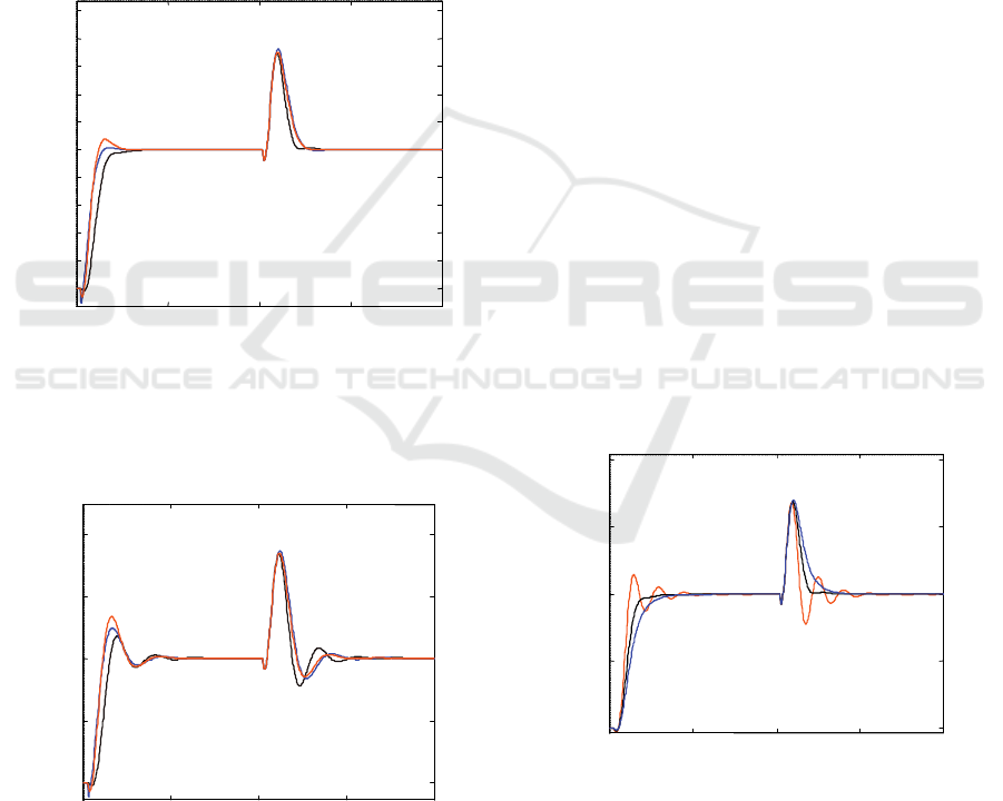
=0.5. Figure 3
illustrates the comparison of the servo-responses as
well as of the regulatory control responses obtained
by the proposed method and by the methods
reported in Chien
et al (2003) and Chen et al (2006),
in the case of nominal process parameters. In case of
set-point tracking, the proposed method provides a
0 20 40 60 80
0
0.2
0.4
0.6
0.8
1
1.2
1.4
1.6
1.8
2
Time (second)
Closed-Loop Response
Figure 3: Servo-responses and regulatory control
responses for the system G
P
(s)=(-0.5s+1)exp(-0.8s)/(s+1),
in case of nominal process parameters. Black line:
Proposed Method. Orange line: Method in Chien et al
(2003). Blue line: Method in Chen et al (2006).
0 20 40 60 80
0
0.5
1
1.5
2
Time (second)
Closed-Loop Response
Figure 4: Servo-responses and regulatory control
responses for the system G
P
(s)=(-0.5s+1)exp(-0.8s)/(s+1),
in case of a +20% mismatch in all process parameters.
Other legend as in Figure 3.
slightly more sluggish response as compared to the
abovementioned PID tuning methods, while the
initial jump obtained by our method is smaller. In
the case of regulatory control, our method gives a
better response in terms of maximum error, while
the settling time is comparable to that obtained by
the methods in Chien
et al (2003) and Chen et al
(2006).
A comparison in terms of the ISE criterion, in the
case of regulatory control, gives the values 1.2002
for the proposed method, while for the methods in
Chien
et al (2003) and Chen et al (2006), we obtain
ISE=1.5782 and ISE=1.4425, respectively. The
respective IAE values for the methods under
comparison are obtained as 2.443, 3.058 and 2.8941.
Figure 4 shows the comparisons of the servo-
responses and of the regulatory control responses in
the case where a simultaneous +20% uncertainty in
all process parameters is assumed. The responses
obtained by the proposed method are better in terms
of overshoot, maximum error and initial jump, while
the settling time is similar to that of the responses
obtained by the PID controllers tuned according to
the methods by Chien
et al (2003) and Chen et al
(2006). The ISE values, in case of regulatory
control, are 1.9514, for the proposed method, 2.3765
for the method of Chien
et al (2003) and 2.1673, for
the method of Chen
et al (2006). The respective IAE
values are 3.8221, 4.2492 and 3.9183.
As already mentioned, for a pre-specified value
of adjustable parameter α, parameter β is directly
related to the damping ration ζ of the second order
approximation (10) of the closed-loop system. In
0 20 40 60 80
0
0.5
1
1.5
2
Time (second)
Closed-Loop Response
Figure 5: Servo-responses and regulatory control
responses for the system G
P
(s)=(-0.5s+1)exp(-0.8s)/(s+1),
in case of nominal process parameters, for α=0.6 and for
three values of β. Orange line: β=2.05; Black line:
β=2.15;. Blue line: β=2.25.
A NEW METHOD OF TUNING THREE TERM CONTROLLERS FOR DEAD-TIME PROCESSES WITH A
NEGATIVE/POSITIVE ZERO
79
0 20 40 60 80 100
0
0.5
1
1.5
2
Time (second)
Closed-Loop Response
Figure 6: Servo-responses and regulatory control
responses for the system G
P
(s)=(-0.5s+1)exp(-0.8s)/(s+1),
in case of nominal process parameters, for β=2 and for
three values of α. Orange line: α=0.45; Black line: α=0.5;.
Blue line: α=0.55.
particular, as shown in Figure 5, β increases when ζ
is increased. This of course results to a more
conservative PD-1F controller. Therefore, a greater
value of β, renders the closed-loop system more
robust. Parameter α has an inverse effect on the
closed-loop system robustness: For a pre-specified
value of the parameter β, an increase of the
parameter α, leads to a less robust but faster closed-
loop system, as illustrated in Figure 6.
4.2 Control of a Continuous Stirred
Tank Reactor
Let us consider the transfer function model of a
CSTR reported in Padma Sree and Chidambaram
(2004), and having the form
P
2
2.07(0.1507s 1)
G(s) exp(0.3s)
2.85s 2.31s 1
2.07(0.1507s 1)
exp( 0.3s)
(0.8905s 1)(3.2005s 1)
−+
=−
+−
−+
=−
+−
The process has one dominant unstable pole and
one stable pole, at s=0.3125 and s= -1.123,
respectively, as well as a stable zero -6.6357. Here,
K=-2.07, τ
1
=0.8905, τ
2
= 3.2005, d=0.3, p=0.1507,
q=-1. Application of the proposed method with α=-
0.5, β=2.5, yields the PD-1F controller settings K
P
=-
4.3862, K
I
=-1.7545, K
d
=-2.2859. The settings of the
set-point weighted PID controller tuned according to
the method reported in Padma Sree and
Chidambaram (2004) are, K
C
=-0.7205, τ
I
=39.7228,
τ
D
=0.1494, while the tuning parameter used in the
above mentioned paper, as well as the set-point
weight b, take the values 0.15 and 0.3275,
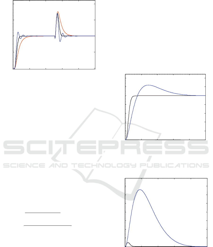
respectively. Figure 7 illustrates the servo-responses
obtained by the two controllers. Figure 8 shows the
comparison of the regulatory control responses for a
negative unit step load change. Obviously, the PD-
1F controller tuned according to the proposed
method provides a considerably better performance,
particularly in the case of regulatory control, where
the response obtained by the controller tuned
according to the method in Padma Sree and
Chidambaram (2004) is practically unacceptable.
0 10 20 30 40 50
0
0.2
0.4
0.6
0.8
1
1.2
1.4
Time (second)
Closed-Loop Response
Figure 7: Closed-loop servo-responses of the CSTR
model. Black line: Proposed method. Blue line: Set-point
weighted PID controller tuned according to the method
proposed by Padma Sree and Chidambaram (2004).
0 10 20 30 40 50
0
0.5
1
1.5
2
2.5
3
3.5
Time (second)
Closed-Loop Response
Figure 8: Regulatory control responses of the CSTR.
Other legend as in Figure 7.
ICINCO 2009 - 6th International Conference on Informatics in Control, Automation and Robotics
80
4.3 Second Order Unstable Process
with a Positive Zero
Consider the process with K=1, τ
1
=2.07, τ
2
=5,
d=0.939, p=-1, q=-1. The process has a stable pole,
an unstable pole and a strong non-minimum phase
zero. To the authors’ best knowledge, controller
design for second order processes with one or two
righ-half-plane poles and a right-half-plane zero has
not yet been addressed in the literature. Application
of the proposed method, with α=0.3 and β=25, yields
the PD-1F controller settings K
I
=0.0920, K
P
=2.3012,
K
d
=4.9027. The process model is next approximated
as
(
)
(
)
P
G (s) exp( 1.939s) / 2.07s 1 5s 1=− + −
⎡
⎤
⎣
⎦
, i.e.
the negative numerator time constant has been
approximated as a time delay term of the form exp(-
s). This is reasonable since an inverse response has a
deteriorating effect on control similar to that of a
time delay. We next apply the method reported in
Lee
et al (2000), in order to design a PID controller
with first order set-point filter for the given process,
on the basis of the approximated model. Application
of the method reported in Lee
et al (2000), with the
IMC parameter λ=6.25, yields the PID controller
settings K
C
=1.9570, τ
Ι
=34.9614 and τ
D
=2.4889.
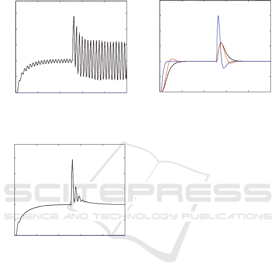
Figure 9 illustrates the comparison of the servo-
responses and the regulatory control responses for a
unit step set-point change at t=0 sec and an inverse
unit step load change at t=75 sec. It is seen that the
proposed method results in an improved load
disturbance response as compared to the method in
Lee
et al (2000), while the set-point responses are
similar, with comparable settling times.
0 50 100 150
0
0.2
0.4
0.6
0.8
1
1.2
Time (second)
Closed-Loop Response
Figure 9: Servo-responses and regulatory control
responses for the system G(s)=(-s+1)exp(-0.939s) /
[(2.07s+1)(5s-1)]. Black line: Proposed method; Blue line:
Method in Lee et al (2000).
4.4 Stable Second Order Unstable
Process with a Positive Zero
Consider the process model of the form (2), with
K=1, τ
1
=2, τ
2
=1, d=1, p=0.3, q=1. Application of the
proposed method with α=0.4, β=3, yields Κ
Ι
=1.0358,
K
P
=3.1073, K
d
=1.6340. The settings of the series
form PID controller with filtered derivative, tuned
according the method proposed by Chien
et al
(2003) are K
C
=1.0355, τ
Ι
=2, τ
D
=1, while the low-
pass filter parameter takes the value τ
F
=0.3 and the
inverse of the cyclic frequency of the desired
critically damped closed-loop system takes the value
τ
cl
= d/ 2 = 0.5457. Figure 10 illustrates the
comparison of the servo-responses as well as of the
regulatory control responses obtained by the
proposed method and by the method reported in
Chien
et al (2003). In the regulatory control case our
method gives a considerably better response,
whereas, although our method provides a smooth
response, the method in Chien
et al (2003) is better
in the case of set-point tracking.
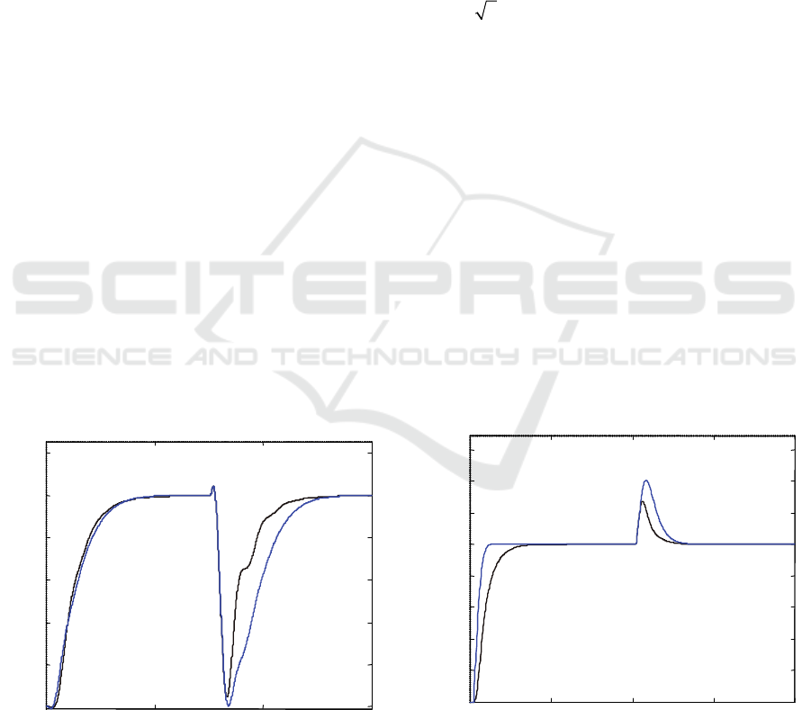
Let us now consider the case of a large overshoot
process with K=1, τ
1
=2, τ
2
=1, d=1.2, p=5, q=1.
Evaluating relations (17)-(19), while assuming
α=0.2, β=3, yields the PD-1F controller settings
K
I
=0.2208, K
P
=0.6624, K
d
= 0.3759. Application of
the above controller yields an unacceptable
oscillatory response, as shown in Figure 11. Let us
try, another design by evaluating relations (17)-(19)
in the case where we select a=0.6, β=3. This yields
K
I
=0.1951, K
P
=0.5853, K
d
= 0.1486, i.e. a more
conservative controller. The obtained servo-response
0 20 40 60 80
0
0.2
0.4
0.6
0.8
1
1.2
1.4
1.6
Time (second)
Closed-Loop Response
Figure 10: Servo-responses and regulatory control
responses for the system G
P
(s)=(0.3s+1)exp(-0.8s)
/(2s+1)(s+1). Black line: Proposed method. Blue line:
Method in Chien et al (2003).
A NEW METHOD OF TUNING THREE TERM CONTROLLERS FOR DEAD-TIME PROCESSES WITH A
NEGATIVE/POSITIVE ZERO
81
0 20 40 60 80 100
0
0.5
1
1.5
2
2.5
Time (second)
Closed-Loop Response
Figure 11: Closed-loop servo-response and regulatory
control response of the system G(s)=(5s+1)exp(-1.2s)
/(2s+1)(s+1), in the case of he PD-1F controller with
parameters K
I
=0.2208, K
P
=0.6624, K
d
= 0.3759.
0 20 40 60 80 100
0
0.5
1
1.5
2
2.5
Time (second)
Closed-Loop Response
Figure 12: Closed-loop servo-response and regulatory
control response of the system G(s)=(5s+1)exp(-1.2s)
/(2s+1)(s+1), in the case of he PD-1F controller with
parameters K
I
=0.1951, K
P
=0.5853, K
d
= 0.1486.
and regulatory control responses are given in Figure
12. In the later case, the servo-response is quite
smooth while the regulatory control response is less
oscillatory. However, the robustness of the closed-
loop system is marginal, and a small parameter
mismatch can readily lead to instability.
Let us now consider filtering the output of the PD-
1F controller that is designed for the case where
α=0.2, β=3, with settings K
I
=0.2208, K
P
=0.6624,
K
d
= 0.3759, by a filter of the form (24), where τ
F
=5.
Moreover, let us design a PD-1F controller with
filtered output as suggested by relations (26)-(28),
with α=-0.2, β=2, τ
F
=5. In this case the controller
0 20 40 60 80 100
0
0.5
1
1.5
2
2.5
Time (second)
Closed-Loop Response
Figure 13: Closed-loop servo-response and regulatory
control responses of the system G(s)=(5s+1)exp(-1.2s)
/(2s+1)(s+1). Black line: PD-1F controller with filtered
output tuned according to relations (17)-(19); Orange line:
PD-1F controller with filtered output tuned according to
relations (26)-(28); Blue line: Series form PID controller
with filtered derivative tuned according to the method in
Chien et al (2003).
settings are K
I
=0.3183, K
P
=0.6366, K
d
= 0.1344.
Figure 13 shows the obtained servo-responses and
regulatory control responses for both designs,
together with the respective responses obtained by a
series PID controller with filtered derivative,
designed according the method reported in Chien
et
al (2003). It is seen that, in the regulatory control
case our method gives a considerably better
response, whereas, although our methods provide
smooth responses, the method in Chien
et al (2003)
is better in the case of set-point tracking. A
comparison in terms of ISE in the case of regulatory
control gives the ISE values 1.8326 and 1.5892, for
the proposed methods and 4.5754 for the method in
Chien
et al (2003). The respective IAE values are
4.5287, 3.7058 and 4.9453.
5 CONCLUSIONS
A new direct synthesis method of tuning the PDF
controller for stable or unstable dead-time processes
with a negative or a positive zero has been
presented. The proposed tuning method ensures
smooth closed-loop response to set-point changes,
fast regulatory control and sufficient robustness
against parametric uncertainty. Numerical
simulation examples verify the advantages of the
proposed method over known PID controller tuning
methods for the classes of dead-time processes under
ICINCO 2009 - 6th International Conference on Informatics in Control, Automation and Robotics
82

study. Extension of the proposed tuning method in
the case of frequency domain specifications of the
closed-loop system in terms of gain and phase
margins is currently under investigation.
REFERENCES
Chang, D.M., Yu, C.C., Chien, I.-L., 1997. Identification
and control of an overshoot lead-lag plant. J. Chin.
Inst. Chem. Eng., 28, 79-89.
Chen, P.-Y., Tang, Y.-C., Zhang, Q.-Z., Zhang, W.-D.,
2005. A new design method of PID controller for
inverse response processes with dead time, Proc. 2005
IEEE Conference on Industrial Technology (ICIT
2005), Hong Kong, China, December 14-17, 2005,
1036-1039.
Chen, P.-Y., Zhang, W.-D., Zhu, L.-Y., 2006. Design and
tuning method of PID controller for a class of inverse
response processes. Proc. 2006 American Control
Conference, Minneapolis, Minnesota, U.S.A., June 14-
16, 2006, 274-279
Chien, I.-L., Chung, Y.-C., Chen B.-S., Chuang, C.-Y.,
2003. Simple PID controller tuning method for
processes with inverse response plus dead time or
large overshoot response plus dead time. Ind. Engg.
Chem. Res., 42, 4461-4477.
Lee, Y.-H., Lee, J.-S., Park, S.-W., 2000. PID controller
tuning for integrating and unstable processes with time
delay. Chem. Engg. Sci., 55, 3481-3493.
Luyben, W.L., 2000. Tuning Proportional-Integral
Controllers for processes with both inverse response
and deadtime. Ind. Eng. Chem. Res., 39, 973-976.
Padma Sree, R., Chidambaram, M., 2004. Simple method
of calculating set point weighting parameter for
unstable systems with a zero. Comp. Chemical Engg.,
28, 2433-2437.
Phelan, R.M., Automatic Control Systems, New York,
Cornell University Press, 1978.
Scali, C., Rachid, A., 1998. Analytical design of
Proportional-Integral-Derivative controllers for
inverse response processes. Ind. Eng. Chem. Res., 37,
1372-1379.
Waller, K.V.T., Nygardas, C.G., 1975. On inverse
response in process control. Ind. Eng. Chem. Fundam.,
14, 221-223.
Zhang, W., Xu, X., Sun, Y., 2000. Quantitative
performance design for inverse-response-processes.
Ind. Eng. Chem. Res., 39, 2056-2061.
A NEW METHOD OF TUNING THREE TERM CONTROLLERS FOR DEAD-TIME PROCESSES WITH A
NEGATIVE/POSITIVE ZERO
83
