A NOVEL VISION-BASED REACTIVE NAVIGATION STRATEGY

BASED ON INVERSE PERSPECTIVE TRANSFORMATION

∗

Francisco Bonin-Font, Alberto Ortiz and Gabriel Oliver

Department of Mathematics and Computer Science, University of the Balearic Islands

Ctra de Valldemossa Km 7.5, 07122, Palma de Mallorca, Spain

Keywords:

Mobile robots, Vision, Obstacle Avoidance, Feature Tracking, Inverse Perspective Transformation, SIFT.

Abstract:

This paper describes a new vision-based reactive navigation strategy addressed to mobile robots, comprising

obstacle detection and avoidance. Most of the reactive vision-based systems base their strength uniquely on

the computation and analysis of quantitative information. The proposed algorithm combines a quantitative

process with a set of qualitative rules to converge in a robust technique to safely explore unknown environ-

ments. The process includes a feature detector/tracker, a new feature classiﬁer based on the Inverse Perspective

Transformation which discriminates between object and ﬂoor points, and a qualitative method to determine

the obstacle contour, their location in the image, and the course that the robot must take. The new strategy has

been implemented on mobile robots with a single camera showing promising results.

1 INTRODUCTION

Visual techniques for detecting and tracking main

scene features have been notably improved over the

last few years and applied to robot navigation solu-

tions. Zhou and Li (Zhou and Li, 2006) detected

ground features grouping all coplanar points that have

been found with the Harris corner detector (Harris and

Stephens, 1988). Lowe (Lowe, 2004) developed the

Scale Invariant Feature Transform (SIFT) method to

extract highly discriminative image features, robust

to scaling, rotation, camera view-point changes and

illumination changes. Rodrigo et al (Rodrigo et al.,

2006) estimated the motion of a whole scene com-

puting a homography matrix for every different scene

plane. Mikolajczyk and Schmid (Mikolajczyk and

Schmid, 2005) compared the performance of differ-

ent descriptors for image local regions showing that,

for different region matching approaches SIFT yields

the best performance in all tests. The Inverse Per-

spective Transformation (IPT) has been successfully

used in obstacle detection procedures. Mallot et al

(Mallot et al., 1991) analyzed variations on the opti-

cal ﬂow computed over the Inverse Perspective Trans-

formation of consecutive frames to detect the pres-

ence of obstacles. Bertozzi and Broggi (Bertozzi and

∗

This work is partially supported by DPI 2008-06548-

C03-02 and FEDER funding.

Broggi, 1997) applied the IPT to project two stereo

images onto the ground. The subtraction of both pro-

jections generate a non-zero pixel zone that evidences

the presence of obstacles. Ma et al (Ma et al., 2007)

presented an automatic pedestrian detector based on

IPT for self guided vehicles. The system predicts new

frames assuming that all image points lie on the ﬂoor,

generating distorted zones that correspond to obsta-

cles.

This paper addresses the problem of obstacle de-

tection and avoidance for a safe navigation in unex-

plored environments. First, image main features are

detected, tracked across consecutive frames, and clas-

siﬁed as obstacles or ground using a new algorithm

based on IPT. Next, the edge map of the processed

frame is computed, and edges comprising obstacle

points are discriminated from the rest of the edges.

This result gives a qualitative idea about the position

of obstacles and free space. Finally, a new version

of the Vector Field Histogram (Borenstein and Koren,

1991) method, here adapted to systems equipped with

visual sensors, is applied to compute a steering vector

which points towards the areas into which the vehicle

can safely move. The rest of the paper is organized as

follows: the method is outlined in Section 2, exper-

imental results are exposed and discussed in Section

3, and ﬁnally, conclusions and forthcoming work are

given in Section 4.

141

Bonin-Font F., Ortiz A. and Oliver G.

A NOVEL VISION-BASED REACTIVE NAVIGATION STRATEGY BASED ON INVERSE PERSPECTIVE TRANSFORMATION.

DOI: 10.5220/0002171301410146

In Proceedings of the 6th International Conference on Informatics in Control, Automation and Robotics (ICINCO 2009), page

ISBN: 978-989-674-000-9

2 THE NEW METHOD

2.1 Inverse Perspective Transformation

The Direct Perspective Transformation is the ﬁrst-

order approximation to the process of taking a picture.

The line that connects a world point with the lens in-

tersects the image plane and deﬁnes its unique image

point. The Inverse Perspective Transformation speci-

ﬁes the straight line upon which the world point cor-

responding to a certain image point must lie. (Hart-

ley and Zisserman, 2003) describes the Direct and In-

verse Perspective Transformation processes and both

are also modeled in (Duda and Hart, 1973), as well as

the expressions to calculate the world coordinates for

points lying on the ﬂoor (z = 0):

x = X

−

cosθ+ (y

sinϕ− fcosϕ)(Z

sinθ)

cosϕ+ f sinϕ

(1)

y = Y

−

sinθ− (y

sinϕ− fcosϕ)(Z

cosθ)

cosϕ+ f sinϕ

(2)

where (x

, y

) are the point image coordinates, (x, y)

are the point world coordinates, (X

) are the lens

world coordinates at the moment in which the frame

has been taken, f is the focal length, and θ and ϕ are

the yaw and pitch angles of the camera, respectively.

2.2 Obstacle and Ground Points

Presuming that all image points lie on the ﬂoor (i.e.

z = 0), their (x,y) world coordinates can be calculated

using (1) and (2). This is an incorrect assumption for

points of obstacles that protrude vertically from the

ﬂoor. As a consequence, the (x, y) world coordinates

(for z = 0) of an obstacle point are different when

they are calculated from two consecutive images, and

different to the obstacle point real (x, y) world coor-

dinates. However, the (x, y) world coordinates (for

z = 0) of a ground point, are equal when they are com-

puted from two consecutive images, and equal to the

real (x, y) ground point world coordinates. Hence, as-

suming z = 0 and analyzing the distance between the

resulting (x, y) point world coordinates for z = 0, cal-

culated across two consecutive images, one can dis-

tinguish if the point belongs to an object or to the

ﬂoor:

D =

− x

)

+ (y

− y

)

⇒

(

ifD > β⇒ obstacle,

ifD ≤ β ⇒ ground .

(3)

where (x

, y

) and (x

) are the (x, y) feature world

coordinates(for z = 0) at instants t

and t

respectively

and β is the threshold for the maximum difference ad-

missible between (x

) and (x

) to consider both

as the same point. Ideally β should be 0.

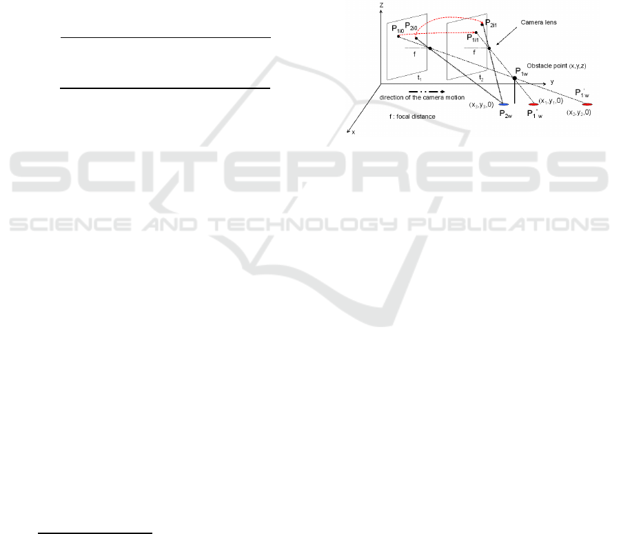
Figure 1 illustrates the idea. Two frames of a scene

are taken at instants t

and t

. Point P

is on the

ground. Its projection into the image plane at instants

and t

generates, respectively, the image points P

2i0

and P

2i1

. The Inverse Transformation of P

2i0

and P

2i1

generates a single point P

. P

is an obstacle point.

Its projection into the image plane at t

and t

gen-

erates, respectively, points P

1i0

and P

1i1

. However,

the projection of P

1i0

and P

1i1

onto the ground plane

( i.e. Inverse Transformation assuming z = 0) gener-

ates two different points on the ground, namely, P

′

and P

′′

Figure 1: The IPM-based obstacle detection principle.

2.3 Feature Detection and Tracking

The ﬁrst step of the obstacle detection algorithm is

to ﬁnd a sufﬁciently large and relevant set of image

points, and establish a correspondence of all these

points between consecutive frames. SIFT features

(Lowe, 2004) have been chosen as the features to

track because of their robustness to scale changes, ro-

tation and/or translation as well as changes in illumi-

nation and view point. In order to ﬁlter out possible

wrong correspondences between points in consecu-

tive frames, outliers are ﬁltered out using RANSAC

and imposing the epipolar constraint. After the de-

tection and tracking process, features are classiﬁed as

ground or obstacle.

Small changes in the distance threshold β can al-

ter the classiﬁcation of those points which have a D

value (3) close to β. In order to decrease the sensitiv-

ity of the classiﬁer with regard to β, all these points

are left unclassiﬁed. Additionally, in a previous train-

ing phase, and for each different scene, histograms of

D values for well classiﬁed and misclassiﬁed points

are built and analyzed. For every different scene, D

values of ground points wrongly classiﬁed as obstacle

are stored in a database. In the autonomousnavigation

phase, all object points with a D value included in that

set of stored D values of the current scene, are neither

ICINCO 2009 - 6th International Conference on Informatics in Control, Automation and Robotics

142

classiﬁed. In this way, nearly all ground points clas-

siﬁed as obstacles are eliminated, reducing the risk of

detecting false obstacles, and although some true ob-

stacle points are also removed, the remaining ones are

sufﬁcient to permit the detection of those obstacles.

2.4 Obstacle Proﬁles and the Navigation

Strategy

SIFT features are usually detected at regions of high

intensity variation (Lowe, 2004) and besides, com-

monly they are near or belong to an edge. Obsta-

cles usually have a high degree of vertical edges and

have one or some points in contact with the ﬂoor. All

detected obstacle points are most likely to be con-

tained or near a vertical edge which must belong to

that obstacle. Hence, the next step of the algorithm is

the computation of the processed images edge map,

and the detection of all complete edges that comprise

real obstacle points. This permits to isolate the ob-

stacle boundaries from the rest of the edges and to

get a qualitative perception of the environment. Ob-

stacle points wrongly classiﬁed as ground can be re-

classiﬁed if they are comprised in an edge that con-

tains other obstacle points.

In order to combine a high degree of performance

in the edge map computation with a relatively low

processing time, our edge detection procedure runs

in two steps (Canny, 1986): a) The original image

is convolved with a 1D gaussian derivative, detecting

zones with high vertical gradient from smoothed in-

tensity values with a single convolution; b) A process

of hysteresis thresholding is applied. Two thresholds

are deﬁned. A pixel with a gray level above the high-

est threshold is classiﬁed as edge pixel. A pixel with

a gray level above the lowest threshold is classiﬁed as

edge if it has in its vicinity a pixel with a gray value

higher than the highest threshold.

The proposed navigation strategy has been in-

spired by (Borenstein and Koren, 1991). Only obsta-

cles detected inside a ROI (Region of Interest) cen-

tered at the bottom of the image are considered to

be avoided. This guarantees a virtual 3-D sphere of

safety around the robot. The image ROI is in turn

divided in angular regions. Those polar directions,

corresponding to angular regions occupied by a real

obstacle boundary are labeled as forbidden and those

free of obstacle boundaries are included in the set

of possible next movement directions. This process

results in a polar map of free and occupied zones.

Obstacle-free polar regions which are narrower than

a certain threshold (determined empirically and de-

pending on the robot size) are excluded from the pos-

sible motion directions. If all angular regions are

narrower than the deﬁned threshold, the algorithm

returns a stop order. The next movement direction

is given as a vector, pointing to the widest polar

obstacle-free zone. Positive angles result for turns to

the right and negative angles for turns to the left. The

computed steering vector qualitatively points towards

the free space and the complete algorithm gives a rea-

sonable idea of whether this free space is wide enough

to continue the navigation through it.

3 EXPERIMENTAL RESULTS

A Pioneer 3Dx mobile robot with a calibrated wide

angle camera was programmed to navigate at 40mm/s

in different environments to test the proposed strat-

egy: environments with obstacles of regular and un-

regular shape, environments with textured and untex-

tured ﬂoor, and environments with specularities or

with low illumination conditions. Operative param-

eter settings: image ROI = 85 pixels; for the hystere-

sis thresholding: low level= 40 and high levels= 50;

camera height= 430mm; ϕ = −9

◦

; initial θ = −2

◦

and ﬁnally, f = 3.720mm. For each scene, the com-

plete navigation algorithm was run over successive

pairs of 0.56-second-separationconsecutiveframes so

that the effect of IPT was noticeable. Increasing the

frame rate decreases the IPT effect over the obstacle

points, and decreasing the frame rate delays the ex-

ecution of the algorithm. Frames were recorded and

down-sampled to a resolution of 256×192 pixels, in

order to reduce the computation time. All frames

were also undistorted to correct the error in the im-

age feature position due to the distortion introduced

by the lens, and thus, to increase the accuracy in the

calculation of the point world coordinates.

In order to assess the classiﬁer performance ROC

curves were computed, deﬁning obstacle points clas-

siﬁed as obstacle as true positives (TP), obstacle

points classiﬁed as ground as false negatives (FN),

ground points classiﬁed as ﬂoor as true negatives

(TN) and ground points classiﬁed as obstacles as false

positives (FP). The AUC (Area Under the Curve)

were calculated as a measure of success classiﬁca-

tion rate, suggesting success rates greater than 93%

(Bonin-Font et al., 2008). The β operational value

(3) was obtained for every scene minimizing the cost

function f(β) = FP(β) + λFN(β). During the ex-

periments, λ was set to 0.5 to prioritize the minimiza-

tion of false positives over false negatives. The value

of f(β) was calculated for every pair of successive im-

ages, changing β. For a varied set of scenes differing

in light conditions and/or ﬂoor texture, the optimum

β had a coincident value of 20mm.

A NOVEL VISION-BASED REACTIVE NAVIGATION STRATEGY BASED ON INVERSE PERSPECTIVE

TRANSFORMATION

143

(a) (b) (c) (d)

(e) (f) (g) (h)

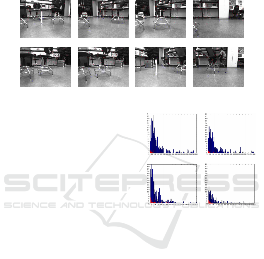
Figure 2: Scene 1. (a) to (d)- Experiment 1. (e) to (h)- Experiment 2: Object and ﬂoor points after the ﬁlter.

Images (a), (b), (c) and (d) of ﬁgure 2 show the

undistorted second frame of several pairs of consecu-

tive images, recorded and processed on-line. Images

show SIFT features classiﬁed as ground (blue) and

classiﬁed as obstacles (red). Every image was taken

just before the robot had to turn to avoid the obstacles

it had in front. Notice that all four pictures present a

few false positives on the ﬂoor.

Histograms of D values for TP (in blue) and FP

(in red) are presented in ﬁgure 3. Plot (a) corre-

sponds to scene 1 (ﬁgure 2), plot (b) to scene 2, plot

Scenes 2,3 and 4 are shown in ﬁgure 4. These his-

tograms count false and true positives for different D

values, in all frames recorded and computed by the

algorithm during a complete sequence. Although his-

tograms belong to environments with different light-

ing conditions or ﬂoor textures, and scenarios with

inter-reﬂections or specularities, results were com-

monly similar: most of the true positives presented

D values between 20mm and 300mm, and the ma-

jority of false positives had D values between 20mm

and approximately 80mm. All positives with D values

between 20mm and 80mm were ﬁltered and left un-

classiﬁed. This ﬁltering process increases AUCs until

the 96%, however, obstacle points near the ﬂoor have

more probabilities of been miss-classiﬁed than others

since their D value can be lower than 20mm.

Pictures (e) to (h) of ﬁgure 2 were taken dur-

ing a second experiment through the environment of

scene 1. In this experiment, the ﬁlter outlined in

the previous paragraph was applied. Notice that all

false positives have been eliminated. This reduces the

risk of detecting false obstacles but maintains a sufﬁ-

cient number of true positives to detect the real obsta-

cles. After the process of feature detection, tracking,

and classiﬁcation, the algorithm localizes every ob-

(a) (b)

Figure 3: Histograms of D values: TP (blue) and FP (red).

ject point in the edge map of the second frame, and

then searches for all edge pixels which are inside a

patch window of 8×13 pixels, centered in the feature

image coordinates. Every edge is tracked down start-

ing from the object point position until the last edge

pixel is found, and considering this last edge pixel to

be the point where the object rests on the ﬂoor. This

process results into the identiﬁcation of the object ver-

tical contours. The consecutive execution of the com-

plete algorithm using successive image pairs as input

results in a collection of consecutive steering vectors

used as the continuous motion orders. After every

robot turn, the value of the camera yaw angle is up-

dated, adding the turn angle to the previousyaw value.

The camera world coordinates are calculated compos-

ing the robot orientation and its center world coordi-

nates obtained via dead reckoning, with the relative

camera position respect to the center of the robot.

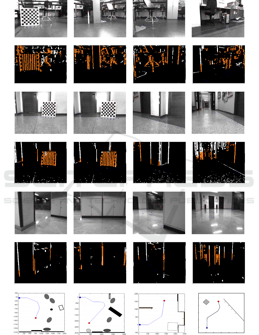
Pictures from (a) to (d), (i) to (l) and (p) to (s)

in ﬁgure 4 show the second frame of different pairs

ICINCO 2009 - 6th International Conference on Informatics in Control, Automation and Robotics

144

of consecutive images, recorded and processed dur-

ing the navigation through the scenarios 2, 3 and 4,

respectively. Every image was taken before the robot

had to turn to avoid the frontal obstacles, and show

obstacle (in red) and ground points (in blue). Scene

2 presents inter-reﬂections, specularities, and a lot of

obstacles with regular and irregular shapes. Scene

3 shows a route through a corridor with a very high

textured ﬂoor, columns and walls. Scene 4 presents

bad illumination conditions, a lot of inter-reﬂections

on the ﬂoor, and some image regions (walls) with al-

most homogeneous intensities and/or textures, which

results in few distinctive features and poorly edged

obstacles. Walls with a very homogeneous texture

and few distinctivefeatures can present difﬁculties for

its detection as an obstacle. In all scenes, all obsta-

cle points with a D value between 20mm and 80mm

were left unclassiﬁed, except in scene 4, where, only

those obstacle points with a D value between 20mm

and 45mm were ﬁltered out. Pictures (e) to (h), (z) to

(o) and (t) to (x) of ﬁgure 4 show the vertical contours

(in orange) comprising obstacle points. See attached

to every picture the angle of the computed steering

vector. For example, in picture (x) objects are out of

the ROI, then, the computed turn angle is 0

◦

(follow

ahead). In picture (e) the obstacles are partially inside

the ROI, so the robot turns to the right (40

◦

). De-

spite scene 4 presents a poor edge map and few SIFT

features, the resulting steering vectors still guide the

robot to the obstacles-free zone. Plots (1) to (4) show

an illustration of the environment and the robot tra-

jectory (blue circle: the starting point; red circle: the

ﬁnal point) for scenes 1, 2, 3 and 4, respectively. In all

scenes, all features were well classiﬁed, obstacle pro-

ﬁles were correctly detected and the robot navigated

through the free space avoiding all obstacles. The

steering vector is computed on the image and then it

is used qualitatively to guide the robot.

4 CONCLUSIONS

This paper introduces a new vision-based reactive

navigation strategy addressed to mobile robots. It

employs an IPT-based feature classiﬁer that distin-

guishes between ground and obstacle points with a

success rate greater than 90%. The strategy was

tested on a robot equipped with a wide angle camera

and showed to tolerate scenes with shadows, inter-

reﬂections, and different types of ﬂoor textures or

light conditions. Experimental results obtained sug-

gested a good performance, since the robot was able

to navigate safely. In order to increase the classiﬁer

success rate, future research includes the evaluation

of the classiﬁer sensitivity to the camera resolution or

focal length. The use of various β values, depending

on the image sector that D is being evaluated, can also

increase the classiﬁer performance.

REFERENCES

Bertozzi, M. and Broggi, A. (1997). Vision-based vehicle

guidance. Computer, 30(7):49–55.

Bonin-Font, F., Ortiz, A., and Oliver, G. (2008).

A novel image feature classiﬁer based on in-

verse perspective transformation. Technical re-

port, University of the Balearic Islands. A-01-2008

(http://dmi.uib.es/fbonin).

Borenstein, J. and Koren, I. (1991). The vector ﬁeld his-

togram - fast obstacle avoidance for mobile robots.

Journal of Robotics and Automation, 7(3):278–288.

Canny, J. (1986). A computational approach to edge detec-

tion. IEEE TPAMI, 8(6):679 – 698.

Duda, R. and Hart, P. (1973). Pattern Classiﬁcation and

Scene Analysis. John Wiley and Sons Publisher.

Harris, C. and Stephens, M. (1988). Combined corner and

edge detector. In Proc. of the AVC, pages 147–151.

Hartley, R. and Zisserman, A. (2003). Multiple view geom-

etry in computer vision. Cambridge University Press,

ISBN: 0521623049.

Lowe, D. (2004). Distinctive image features from scale-

invariant keypoints. International Journal of Com-

puter Vision, 60(2):91–110.

Ma, G., Park, S., Mller-Schneiders, S., Ioffe, A., and Kum-

mert, A. (2007). Vision-based pedestrian detection -

reliable pedestrian candidate detection by combining

ipm and a 1d proﬁle. In Proc. of the IEEE ITSC, pages

137–142.

Mallot, H., Buelthoff, H., Little, J., and Bohrer, S. (1991).

Inverse perspective mapping simpliﬁes optical ﬂow

computation and obstacle detection. Biological Cy-

bernetics, 64(3):177–185.

Mikolajczyk, K. and Schmid, C. (2005). A perfor-

mance evaluation of local descriptors. IEEE TPAMI,

27(10):1615–1630.

Rodrigo, R., Chen, Z., and Samarabandu, J. (2006). Feature

motion for monocular robot navigation. In Proc. of the

ICIA, pages 201–205.

Zhou, J. and Li, B. (2006). Homography-based ground de-

tection for a mobile robot platform using a single cam-

era. In Proc. of the IEEE ICRA, pages 4100–4101.

A NOVEL VISION-BASED REACTIVE NAVIGATION STRATEGY BASED ON INVERSE PERSPECTIVE

TRANSFORMATION

145

(a) (b) (c) (d)

(e) 40

◦

(f) 65

◦

(g) 50

◦

(h) 0

◦

(i) (j) (k) (l)

(z) 0

◦

(m) −41.5

◦

(n) −43.5

◦

(o) 0

◦

(p) (q) (r) (s)

(t) 48

◦

(u) −39

◦

(w) −43.5

◦

(x) 0

◦

stools

cilinder

stools

lockers and shelves

chessboard

stool

vertical plank

stool

lockers

and shelves

chair

chessboard

front door

lab. wood door

door

column

access to corridor

front wall

with locks and

shelves

1500

1000

500

-500

-500 0 500 1000

1500

2000

2500

2000

(1) (2) (3) (4)

Figure 4: (a) to (d) Scene 2, (i) to (l) Scene 3, (p) to (s) Scene 4. (e) to (h), (z) to (o) and (t) to (x), vertical contours of Scene

2, 3 and 4, respectively. (1) to (4): robot trajectories.

ICINCO 2009 - 6th International Conference on Informatics in Control, Automation and Robotics

146