LMI-BASED TRAJECTORY PLANNING FOR CLOSED-LOOP
CONTROL OF ROBOTIC SYSTEMS WITH VISUAL FEEDBACK
Graziano Chesi
Department of Electrical and Electronic Engineering, University of Hong Kong
Pokfulam Road, Hong Kong, China
Keywords:
Robot control, Visual feedback, Trajectory planning, LMI.
Abstract:
Closed-loop robot control based on visual feedback is an important research area, with useful applications in
various fields. Planning the trajectory to be followed by the robot allows one to take into account multiple
constraints during the motion, such as limited field of view of the camera and limited workspace of the robot.
This paper proposes a strategy for path-planning from an estimate of the point correspondences between the
initial view and the desired one, and an estimate of the camera intrinsic parameters. This strategy consists
of generating a parametrization of the trajectories connecting the initial location to the desired one via poly-
nomials. The trajectory constraints are then imposed by using suitable relaxations and LMIs (linear matrix
inequalities). Some examples illustrate the proposed approach.
1 INTRODUCTION
An important research area in robotics is represented
by visual servoing. This area studies the application
of closed-loop control in robotic system with visual
feedback. Specifically, the problem consists of steer-
ing a robot end-effector from an unknown initial lo-
cation to an unknown desired location by using the
visual information provided by a camera. This cam-
era is typically mounted on the robot end-effector,and
the configuration is known as eye-in-hand configura-
tion. The camera is firstly located at a certain loca-
tion, called desired location, and the image projec-
tions of some object points visible from this location
are recorded. Then, the camera is moved to another
location of the robot workspace, from which the same
object points are visible, and whose relative motion
with respect to the desired location is unknown. The
problem, hence, consists of reaching again the de-
sired location from this new location, which is called
initial location. See for instance (Hashimoto, 1993;
Chaumette and Hutchinson, 2006; Chaumette and
Hutchinson, 2007) and references therein.
The procedure just described is known as
teaching-by-showing approach. It is well-known that
the teaching-by-showing approach has numerous and
various applications, for example in the industrial
manufacture for the construction of complex compo-
nents such as parts of a ship, where its function con-
sists of allowing a robotic arm to grasp and position
tools and objects. Other applications are in surveil-
lance, where a mobile camera observes some areas of
interest such as the entrance of a building in order to
identify people, and in airplane alignment, where the
system to be positioned is represented by the airplane
that has to be aligned with respect to the runway in or-
der to land. Also, the teaching-by-showing approach
finds application in surgery, where an instrument is
automatically guided to the organ to operate, in nav-
igation, where a mobile robot has to explore a scene,
and in dangerous environments such as nuclear sta-
tions and spatial missions, where humans should be
replaced.
In last years, various methods have been devel-
oped for addressing this approach. Some of these
methods have proposed the use of the camera pose
as feedback information (known as position-based
visual servoing, see e.g. (Thuilot et al., 2002)),
definition of the feedback error in the image do-
main (known as image-based visual servoing, see e.g.
(Hashimoto et al., 1991)), use of both camera pose
error and image error (known as 2 1/2 D visual ser-
voing, see e.g. (Malis et al., 2003)), partition of the
degrees of freedoms (Corke and Hutchinson, 2001),
switching strategies for ensuring constraints and im-
proving performance (Chesi et al., 2004; Gans and
Hutchinson, 2007; Lopez-Nicolas et al., 2007), gen-
eration of circular-like trajectories for minimizing the
13
Chesi G.
LMI-BASED TRAJECTORY PLANNING FOR CLOSED-LOOP CONTROL OF ROBOTIC SYSTEMS WITH VISUAL FEEDBACK.
DOI: 10.5220/0002172200130020
In Proceedings of the 6th International Conference on Informatics in Control, Automation and Robotics (ICINCO 2009), page
ISBN: 978-989-674-000-9
Copyright
c
 2009 by SCITEPRESS – Science and Technology Publications, Lda. All rights reser ved

trajectory length (Chesi and Vicino, 2004), control in-
variant to intrinsic parameters (Malis, 2004), use of
complex image features via image moments (Tahri
and Chaumette, 2005), global motion plan via naviga-
tion functions (Cowanand Chang, 2005), use of cylin-
drical coordinate systems (Iwatsuki and Okiyama,
2005), enlargement of stability regions (Tarbouriech
et al., 2005), and model-less control (Miura et al.,
2006).
Path-planning strategies have also been proposed
in order to take into account multiple constraints, such
as limited field of view of the camera and limited
workspace of the robot. See for instance (Mezouar
and Chaumette, 2002; Park and Chung, 2003; Deng
et al., 2005; Allotta and Fioravanti, 2005; Yao and
Gupta, 2007; Kazemi et al., 2009) and references
therein. These methods generally adopt potential
fields along a reference trajectory in order to fulfill the
required constraints, in particular the potential fields
do not affect the chosen reference trajectory wher-
ever the constraints are not violated, while they make
the camera deviating from this path wherever a con-
straint does not hold. The planned trajectory is then
followed by tracking the image projection of this tra-
jectory through an image-based controller such as the
one proposed in (Mezouar and Chaumette, 2002).
In this paper we propose the use of a parametriza-
tion of the trajectories connecting the initial location
to the desired one, together with the use of dedicated
optimization techniques for identifying the trajecto-
ries which satisfy the required constraints. Specif-
ically, this parametrization is obtained by estimat-
ing the camera pose existing between these two lo-
cations and by estimating the position of the object
points in the three-dimensional space. These estima-
tions are performed by exploiting the available im-
age point correspondences between the initial and de-
sired views, and by exploiting the available estimate
of the camera intrinsic parameters. Then, typical tra-
jectory constraints such as the limited field of view
of the camera and the limited workspace of the robot,
are formulated in terms of positivity of certain poly-
nomials. The positivity of these polynomials is then
imposed by using some suitable relaxations for con-
strained optimization. These relaxations can be for-
mulated in terms of LMIs (linear matrix inequalities),
whose feasibility can be checked via convex program-
ming tools. Some examples are reported to illustrate
the application of the proposed approach.
This paper extends our previous works (Chesi and
Hung, 2007), where a path-planning method based on
the computation of the roots of polynomials was pro-
posed (the advantage with respect to this method is
the use of LMIs), and (Chesi, 2009b), where a plan-
ning strategy is derived by using homogeneous forms
(the advantage with respect to this method is the use
of more general relaxations which may allow one to
take into account more complex constraints).
The organization of the paper is as follows. Sec-
tion 2 introduces the notation, problem formulation,
and some preliminaries about representation of poly-
nomials. Section 3 describes the proposed strategy for
trajectory planning. Section 4 illustrates the simula-
tion and experimental results. Lastly, Section 5 pro-
vides some final remarks.
2 PRELIMINARIES
In this section we introduce some preliminaries,
namely the notation, problem formulation, and a tool
for representing polynomials.
2.1 Notation and Problem Formulation
Let us start by introducing the notation adopted
throughout the paper:
- R: real numbers space;
- 0
n
: n × 1 null vector;
- I
n
: n × n identity matrix;
- kvk: euclidean norm of vector v.
We consider a generic stereo vision system, where
two cameras are observing a common set of object
points in the scene. The symbols F
ini
and F
des
repre-
sent the frames of the camera in the initial and desired
location respectively. These frames are expressed as
F
ini
= {R
ini
,t
ini
}
F
des
= {R
des
,t
des
}
(1)
where R
ini
,R
des
∈ R
3×3
are rotation matrices, and
t
ini
,t
des
∈ R
3
are translation vectors. These quanti-
ties R
ini
, R
des
, t
ini
and t
des
are expressed with respect
to an absolute frame, which is indicated by F
abs
.
The observed object points project on the image
plane of the camera in the initial and desired location
onto the image points p
ini
1
,. .. , p
ini
n
∈ R
3
(initial view)
and p
des
1
,. .. , p
des
n
∈ R
3
(desired view). These image
points are expressed in homogeneous coordinates ac-
cording to
p
ini
i
=


p
ini
i,1
p
ini
i,2
1


, p
des
i
=


p
des
i,1
p
des
i,2
1


. (2)
where p
ini
i,1
, p
des
i,1
∈ R are the components on the x-axis
of the image screen, while p
ini
i,2
, p
des
i,2
∈ R are those on
ICINCO 2009 - 6th International Conference on Informatics in Control, Automation and Robotics
14

the y-axis. The projections p
ini
i
and p
des
i
are deter-
mined by the projective law
d
ini
i
p
ini
i
= KR
ini
′

q
i
− t
ini

d
des
i
p
des
i
= KR
des
′

q
i
− t
des

(3)
where d
ini
i
,d
des
i
∈ R are the depths of the ith point,
q
i
∈ R
3
is the ith point expressed with respect to F
abs
,
and K ∈ R
3×3
is the upper triangular matrix contain-
ing the intrinsic parameters of the camera.
The problem we consider in this paper consists of
planning a trajectory from the initial location F
ini
to
the desired one F
des
(which are unknown) by using
the available estimates of:
1. the image projections ˆp
ini
1
, ˆp
des
1
,. .. , ˆp
ini
n
, ˆp
des
n
;
2. and intrinsic parameters matrix
ˆ
K.
This trajectory must ensure that the object points are
kept inside the field of view of the camera, and that
the camera does not exit its allowed workspace.
In the sequel, we will indicate the set of rotation
matrices in R
3×3
as SO(3), and the set of frames in
the three-dimensionalspace as SE(3), where SE(3) =
SO(3) × R
3
.
2.2 Representation of Polynomials
Before proceeding, let us briefly introduced a tool for
representing polynomials which will be exploited in
the sequel. Let p(x) be a polynomial of degree 2m in
the variable x = (x
1
,. .. ,x
n
)
′
∈ R
n
, i.e.
p(x) =
∑
i
1
+ ... + i
n
≤ 2m
i
1
≥ 0,. . . , i
n
≥ 0
c
i
1
,...,i
n
x
i
1
1
·· · x
i
n
n
(4)
for some coefficients c
i
1
,...,i
n
∈ R. Then, p(x) can be
expressed as
p(x) = x
{m}
′
P(α)x
{m}
(5)
where x
{
m}
is any vector containing a base for the
polynomials of degree m in x, and hence can be sim-
ply chosen as the set of monomials of degree less than
or equal to m in x, for example via
x
{
m}
= (1, x
1
,. . . , x
n
,x
2
1
,x
1
x
2
,. . . , x
m
n
)
′
, (6)
and
P(α) = P+ L(α) (7)
where P = P
′
is a symmetric matrix such that
p(x) = x
{m}
′
Px
{m}
, (8)
while L(α) is a linear parametrization of the linear
space
L (n, m) = {L = L
′
: x
{m}
′
Lx
{m}
= 0 ∀x} (9)
being α a vector of free parameters. The dimension
of x
{m}
is given by
σ(n,m) =
(n+ m)!
n!m!
(10)
while the dimension of α (i.e., the dimension of L ) is
τ(n,m) =
1
2
σ(n,m)(σ(n,m) + 1) − σ(n,2m). (11)
The representation in (5) was introduced in (Chesi
et al., 1999) with the name SMR (square matricial
representation). The matrices P and P(α) are known
as SMR matrices of p(x), and can be computed via
simple algorithms. See also (Chesi et al., 2003; Chesi
et al., 2009).
The SMR was introduced in (Chesi et al., 1999)
in order to investigate positivity of polynomials via
convex optimizations. Indeed, p(x) is clearly positive
if it is a sum of squares of polynomials, and this latter
condition holds if and only if there exists α such that
P(α) ≥ 0 (12)
which is an LMI (linear matrix inequality). It turns
out that, establishing whether an LMI admits a feasi-
ble solution or not, amounts to solving a convex opti-
mization.
3 TRAJECTORY PLANNING
This section describes the proposed approach. Specif-
ically, we first introduce the adopted parametrization
of the trajectories, then we describe the computation
of the trajectory satisfying the required constraints,
and lastly we explain how the camera pose and ob-
ject points can be estimated from the available data.
3.1 Trajectory Parametrization
Let us start by parameterizing the trajectory of the
camera from the initial location to the desired one.
This can be done by denoting the frame of the camera
along the trajectory as
F(a) = {R(a),t(a)} (13)
where a ∈ [0,1] is the normalized trajectory abscise,
R(a) ∈ SO(3) is the rotation matrix of F(a), and
t(a) ∈ R
3
is the translation vector. We choose the con-
vention
a = 0 → F(a) = F
ini
a = 1 → F(a) = F
des
.
(14)
The functions R : [0,1] → SO(3) and t : [0,1] → R
3
must satisfy the boundary conditions
R(0) =
ˆ
R
ini
, R(1) =
ˆ
R
des
t(0) =
ˆ
t
ini
, t(1) =
ˆ
t
des
(15)
LMI-BASED TRAJECTORY PLANNING FOR CLOSED-LOOP CONTROL OF ROBOTIC SYSTEMS WITH VISUAL
FEEDBACK
15

where
ˆ
R
ini
,
ˆ
R
des
,
ˆ
t
ini
and
ˆ
t
des
are the available esti-
mates of R
ini
, R
des
, t
ini
and t
des
(the computation of
these estimates will be addressed in Section 3.3). We
adopt polynomials in order to parameterize R(a) and
t(a). Specifically, we parameterize t(a) according to
t(a) =
δ
∑
i=0
ˇ
t
i
a
i
(16)
where δ is an integer representing the chosen degree
for t(a), and
ˇ
t
0
,. . .,
ˇ
t
δ
∈ R
3
are vectors to be deter-
mined. Then, we parameterize R(a) as
R(a) =
E(r(a))
kr(a)k
2
(17)
where E : R
4
→ SO(3) is the parametrization of a ro-
tation matrix via Euler parameters, which is given by
E(r) =


r
2
1
− r
2
2
− r
2
3
+ r
2
4
2(r
1
r
2
− r
3
r
4
)
2(r
1
r
2
+ r
3
r
4
) −r
2
1
+ r
2
2
− r
2
3
+ r
2
4
2(r
1
r
3
− r
2
r
4
) 2(r
2
r
3
+ r
1
r
4
)
2(r
1
r
3
+ r
2
r
4
)
2(r
2
r
3
− r
1
r
4
)
−r
2
1
− r
2
2
+ r
2
3
+ r
2
4


(18)
while r : [0,1] ∈ R
4
denotes the Euler parameter along
the trajectory. It turns out that
E(r) ∈ SO(3) ∀r ∈ R
4
\ {0
4
}, (19)
and moreover
∀R ∈ SO(3) ∃ξ(R) ∈ R
4
\ {0
4
} : E(ξ(R)) = R, (20)
in particular
ξ(R) =



sin
θ
2
u
cos
θ
2



(21)
where θ ∈ [0,π] and u ∈ R
3
, kuk = 1, are respectively
the rotation angle and axis in the exponential coordi-
nates of R, i.e.
R = e
[θu]
×
. (22)
We parameterize r(a) according to
r(a) =
γ
∑
i=0
ˇr
i
a
i
(23)
where ˇr
0
,. . . , ˇr
γ
∈ R
4
are vectors for some integer γ.
The boundary conditions in (15) become, hence,
ˇr
0
= ξ(
ˆ
R
ini
),
∑
γ
i=0
ˇr
i
= ξ(
ˆ
R
des
)
ˇ
t
0
=
ˆ
t
ini
,
∑
δ
i=0
ˇ
t
i
=
ˆ
t
des
(24)
which imply that r(a) and t(a) can be re-
parameterized as
r(a) =

ξ(
ˆ
R
des
) − ξ(
ˆ
R
ini
) −
∑
γ−1
i=1
¯r
i

a
γ
+
∑
γ−1
i=1
¯r
i
a
i
+ ξ(
ˆ
R
ini
)
t(a) =

ˆ
t
des
−
ˆ
t
ini
−
∑
δ−1
i=1
¯
t
i

a
δ
+
∑
δ−1
i=1
¯
t
i
a
i
+
ˆ
t
ini
(25)
where ¯r
1
,. . . , ¯r
γ−1
∈ R
4
and
¯
t
1
,. . .,
¯
t
δ−1
∈ R
3
are free
vectors.
Let us observe that the derived parametrization
can describe arbitrarily complicated trajectories, sim-
ply by selecting sufficiently large degrees γ and δ.
Moreover, it is useful to observe that special cases
such as straight lines are simply recovered by the
choices
γ = 1 (straight line in the domain of E)
δ = 1 (straight line in the translational space).
(26)
For ease of description we will assume γ = 1 in the
following sections.
3.2 Trajectory Computation
In this section we address the problem of identifying
which trajectories inside the introduced parametriza-
tion satisfy the required trajectory constraints. Due
to space limitation, we describe only two fundamen-
tal constraints, in particular the visibility constraint
(the object points must remain in the field of view of
the camera) and the workspace constraint (the cam-
era cannot exit from its allowed workspace). Other
constraints can be similarly considered.
Let us indicate with p
i
(a) = (p
i,1
(a), p
i,2
(a),1)
′
∈
R
3
the image projection of the ith object point along
the trajectory. The visibility constraint is fulfilled
whenever
p
i, j
(a) ∈ (s
i,1
,s
i,2
) ∀i = 1,... , n ∀ j = 1,2 ∀a ∈ [0,1]
(27)
where s
1,1
,s
1,2
,s
2,1
,s
2,2
∈ R are the screen limits. We
estimate p
i
(a) via
p
i
(a) =
f
i
(a)
f
i,3
(a)
+ (1− a)

ˆp
ini
i
−
f
i
(0)
f
i,3
(0)

+a

ˆp
des
i
−
f
i
(1)
f
i,3
(1)

(28)
where f
i
(a) = ( f
i,1
(a), f
i,2
(a), f
i,3
(a))
′
∈ R
3
is
f
i
(a) =
ˆ
KE(r(a))
′
( ˆq
i
− t(a)) (29)
and ˆq
i
∈ R
3
is the estimate of the object point q
i
(the
computation of this estimate will be addressed in Sec-
tion 3.3). Let us observe that this choice ensures
ICINCO 2009 - 6th International Conference on Informatics in Control, Automation and Robotics
16

p
i
(0) = ˆp
ini
i
and p
i
(1) = ˆp
des
i
. We can rewrite p
i
(a) as
p
i
(a) =
1
f
i,3
(a)


g
i,1
(a)
g
i,2
(a)
f
i,3
(a)


(30)
where g
i,1
(a),g
i,2
(a) ∈ R are polynomials.
Then, let us consider the workspace constraint. A
possible way to define the workspace constraint is via
inequalities such as
d
′
i
(t(a
i
) − o
i
) > w
i
∀i = 1,.. .,n
w
(31)
where d
i
∈ R
3
is the direction along which the con-
straint is imposed, a
i
∈ [0,1] specifies where the con-
straint is imposed on the trajectory, o
i
∈ R
3
locates
the constraint, w
i
∈ R specifies the minimum distance
allowed from the point o
i
along the direction d
i
, and
n
w
is the number of constraints.
Hence, let us define the set of polynomials
H =

s
j,k
f
i,3
(a) − (−1)
k
g
i, j
(a) ∀i = 1,.. . ,n,
j, k = 1,2} ∪ { f
i,3
(a) ∀i = 1,.. . ,n}
∪{d
′
i
(t(a
i
) − o
i
) − w
i
∀i = 1,.. . ,n
w
}.
(32)
The visibility and workspace constraints are hence
fulfilled whenever
h(a) > 0 ∀h(a) ∈ H ∀a ∈ [0,1]. (33)
For each polynomial h(a) in H , let us introduce an
auxiliary polynomial u
h
(a) of some degree, and let us
define
v
h
(a) = h(a) − a(1− a)u
h
(a). (34)
Let us express these polynomials via the SMR as
u
h
(a) = y
h
(a)
′
U
h
y
h
(a)
v
h
(a) = z
h
(a)
′
V
h
(α
h
)z
h
(a)
(35)
where y
h
(a),z
h
(a) are vectors containing polynomial
bases, and U,V(α
h
) are symmetric SMR matrices
(see Section 2.2 for details). It can be verified that
(33) holds whenever the following set of LMIs is sat-
isfied:
U
h
> 0
V
h
(α
h
) > 0

∀h(a) ∈ H . (36)
The LMI feasibility test (36) providesa sufficient con-
dition for the existence of a trajectory satisfying the
required constraints. Hence, it can happen that this
condition is not satisfied even if a trajectory does ex-
ist. However, it should be observed that the conser-
vatism of this condition decreases by increasing the
degree of the polynomials used to parameterize the
trajectory.
3.3 Camera Pose and Scene Estimation
In the previous sections we have described how the
trajectory of the camera can be parameterized and
computed. In particular, the parametrization was
based on the estimates
ˆ
R
ini
,
ˆ
R
des
,
ˆ
t
ini
and
ˆ
t
des
of the
components of the initial and desired frames F
ini
and
F
des
, while the computation was based on the esti-
mates ˆq
1
,. . . , ˆq
n
of the object points q
1
,. . . , q
n
. Here
we describe some ways to obtain these estimates.
Given the estimates ˆp
ini
1
, ˆp
des
1
,. . . , ˆp
ini
n
, ˆp
des
n
of the
image projections and
ˆ
K of the intrinsic parameters
matrix, one can estimate the camera pose between
F
ini
and F
des
, and hence R
ini
and t
ini
since F
des
can
be chosen without loss of generality equal to F
abs
.
This estimation can be done, for example, through the
essential matrix or through the homography matrix,
see for instance (Malis and Chaumette, 2000; Chesi
and Hashimoto, 2004; Chesi, 2009a) and references
therein.
Once that the estimates
ˆ
R
ini
and
ˆ
t
ini
have been
found, one can compute the estimates ˆq
1
,. . . , ˆq
n
of
the object points via a standard triangulation scheme,
which amounts to solving a linear least-squares prob-
lem.
Let us observe that, if no additional information is
available, the translation vector and the object points
can be estimated only up to a scale factor. In this case,
the workspace constraint has to be imposed in a nor-
malized space. This problem does not exist if a CAD
model of the object (or part of it) is available, since
this allows to estimate the distance between the ori-
gins of F
ini
and F
des
.
4 ILLUSTRATIVE EXAMPLES
In this section we present some illustrative examples
of the proposed approach. Let us consider the situ-
ation shown in Figure 1a, where a camera observes
some object points (the centers of the nine large dots
in the “2”, “3” and ”4” faces of the three dices) from
the initial and desired locations (leftmost and right-
most cameras respectively). Figure 1b shows the im-
age projections of these points in the initial view (“o”
marks) and desired view (“x” marks). The intrinsic
parameters matrix is chosen as
K =


400 0 320
0 300 240
0 0 1


. (37)
The problem consists of planning a trajectory from
the initial location to the desired one which ensures
that the object points are kept inside the field of view
LMI-BASED TRAJECTORY PLANNING FOR CLOSED-LOOP CONTROL OF ROBOTIC SYSTEMS WITH VISUAL
FEEDBACK
17

of the camera and the camera does not collide with
the sphere interposed between F
ini
and F
des
(which
represents an obstacle to avoid).
Let us use the proposed approach. We parame-
terize the trajectory as described in Section 3.1 with
polynomials of degree two by estimating the camera
pose between F
ini
and F
des
via the essential matrix.
Then, we build the set of polynomials H , which im-
pose the visibility and workspace constraints. The
workspace constraint is chosen by requiring that the
trajectory must remain at a certain distance from the
obstacle in two directions. Hence, we compute the
SMR matrices U
h
and V
h
(α
h
) in (35), and by using
the LMI toolbox of Matlab we find that the LMIs in
(36) are feasible, in particular the obtained feasible
trajectory is shown in Figures 1a and 1b.
−25
−20
−15
−10
−5
0
0
10
20
30
−5
0
5
x [m]
y [m]
z [m]
(a)
0 100 200 300 400 500 600
0
50
100
150
200
250
300
350
400
450
screen x-axis
screen y-axis
(b)
Figure 1: (a) Initial frame F
ini
(leftmost camera), desire
frame F
des
(rightmost camera), object points (centers of the
nine large dots in the “2”, “3” and ”4” faces of the three
dices), planned trajectory (solid line), and some interme-
diate locations of the camera along the planned trajectory.
(b) Image projections of the object points in the initial view
(“o” marks) and desired view (“x” marks), and image pro-
jection of the planned trajectory (solid line).
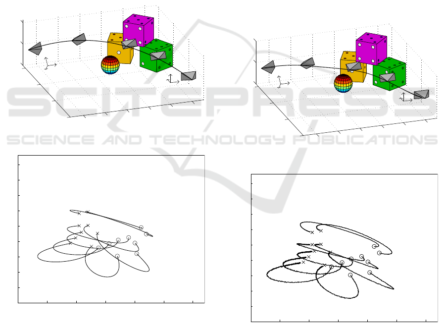
Now, in order to introduce typical uncertainties
of real experiments, we corrupt the image projections
of the object points by adding image noise with uni-
form distribution in [−1,1] pixels to each component.
Moreover, we suppose that the camera is coarsely cal-
ibrated, in particular the available estimate of the in-
trinsic parameters matrix is
ˆ
K =


430 0 338
0 275 250
0 0 1


. (38)
We repeat the previous steps in the presence of
these uncertainties, and then we track the planned tra-
jectory by using the image-based controller proposed
in (Mezouar and Chaumette, 2002). Figures 2a and
2b show the obtained results: as we can see, the cam-
era reaches the desired location by avoiding collisions
with the obstacle in spite of the introduced uncertain-
ties.
−25
−20
−15
−10
−5
0
0
10
20
30
−5
0
5
x [m]
y [m]
z [m]
(a)
0 100 200 300 400 500 600
0
50
100
150
200
250
300
350
400
450
screen x-axis
screen y-axis
(b)
Figure 2: Results obtained by planning the trajectory with
image noise and calibration errors, and by tracking the
planned trajectory with an image-based controller.
Lastly, we consider a more difficult case by in-
troducing three obstacles as shown in Figure 3a. We
ICINCO 2009 - 6th International Conference on Informatics in Control, Automation and Robotics
18

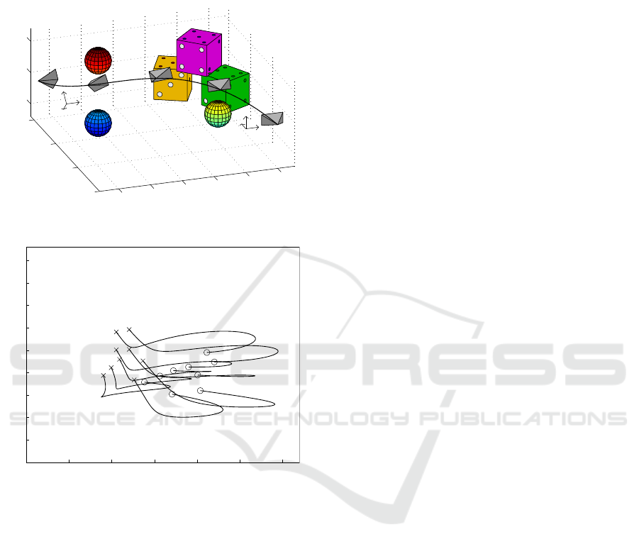
find that the LMIs are feasible by using polynomials
of degree three, and the found solution provides the
trajectory shown in Figures 3a and 3b, which satisfies
the required constraints.
−25
−20
−15
−10
−5
0
0
10
20
30
−5
0
5
x [m]
y [m]
z [m]
(a)
0 100 200 300 400 500 600
0
50
100
150
200
250
300
350
400
450
screen x-axis
screen y-axis
(b)
Figure 3: Results obtained for a different set of obstacles.
5 CONCLUSIONS
We have proposed a trajectory planning strategy for
closed-loop control of robotic systems with visual
feedback, which allows one to take into account mul-
tiple constraints during the motion such as limited
field of view of the camera and limited workspace
of the robot. This strategy is based on generating a
parametrization of the trajectories connecting the ini-
tial location to the desired one. The trajectory con-
straints are imposed by using polynomial relaxations
and LMIs. Future work will investigate the applica-
tion of the proposed approach in real experiments.
ACKNOWLEDGEMENTS
The author would like to thank the Reviewers for
their time and useful comments. This work was
supported by the Research Grants Council of Hong
Kong Special Administrative Region under Grant
HKU711208E.
REFERENCES
Allotta, B. and Fioravanti, D. (2005). 3D motion planning
for image-based visual servoing tasks. In Proc. IEEE
Int. Conf. on Robotics and Automation, Barcelona,
Spain.
Chaumette, F. and Hutchinson, S. (2006). Visual servo con-
trol, part I: Basic approaches. IEEE Robotics and Au-
tomation Magazine, 13(4):82–90.
Chaumette, F. and Hutchinson, S. (2007). Visual servo con-
trol, part II: Advanced approaches. IEEE Robotics and
Automation Magazine, 14(1):109–118.
Chesi, G. (2009a). Camera displacement via con-
strained minimization of the algebraic error. IEEE
Trans. on Pattern Analysis and Machine Intelligence,
31(2):370–375.
Chesi, G. (2009b). Visual servoing path-planning via homo-
geneous forms and LMI optimizations. IEEE Trans.
on Robotics, 25(2):281–291.
Chesi, G., Garulli, A., Tesi, A., and Vicino, A. (2003).
Solving quadratic distance problems: an LMI-based
approach. IEEE Trans. on Automatic Control,
48(2):200–212.
Chesi, G., Garulli, A., Tesi, A., and Vicino, A. (2009). Ho-
mogeneous Polynomial Forms for Robustness Analy-
sis of Uncertain Systems. Springer (in press).
Chesi, G. and Hashimoto, K. (2004). A simple technique for
improving camera displacement estimation in eye-in-
hand visual servoing. IEEE Trans. on Pattern Analysis
and Machine Intelligence, 26(9):1239–1242.
Chesi, G., Hashimoto, K., Prattichizzo, D., and Vicino, A.
(2004). Keeping features in the field of view in eye-
in-hand visual servoing: a switching approach. IEEE
Trans. on Robotics, 20(5):908–913.
Chesi, G. and Hung, Y. S. (2007). Global path-planning for
constrained and optimal visual servoing. IEEE Trans.
on Robotics, 23(5):1050–1060.
Chesi, G., Tesi, A., Vicino, A., and Genesio, R. (1999). On
convexification of some minimum distance problems.
In 5th European Control Conf., Karlsruhe, Germany.
Chesi, G. and Vicino, A. (2004). Visual servoing for
large camera displacements. IEEE Trans. on Robotics,
20(4):724–735.
Corke, P. I. and Hutchinson, S. (2001). A new partitioned
approach to image-based visual servo control. IEEE
Trans. on Robotics and Automation, 17(4):507–515.
Cowan, N. J. and Chang, D. E. (2005). Geometric visual
servoing. IEEE Trans. on Robotics, 21(6):1128–1138.
LMI-BASED TRAJECTORY PLANNING FOR CLOSED-LOOP CONTROL OF ROBOTIC SYSTEMS WITH VISUAL
FEEDBACK
19

Deng, L., Janabi-Sharifi, F., and Wilson, W. J. (2005).
Hybrid motion control and planning strategy for vi-
sual servoing. IEEE Trans. on Industrial Electronics,
52(4):1024–1040.
Gans, N. and Hutchinson, S. (2007). Stable visual servoing
through hybrid switched-system control. IEEE Trans.
on Robotics, 23(3):530–540.
Hashimoto, K. (1993). Visual Servoing: Real-Time Con-
trol of Robot Manipulators Based on Visual Sensory
Feedback. World Scientific, Singapore.
Hashimoto, K., Kimoto, T., Ebine, T., and Kimura, H.
(1991). Manipulator control with image-based visual
servo. In Proc. IEEE Int. Conf. on Robotics and Au-
tomation, pages 2267–2272.
Iwatsuki, M. and Okiyama, N. (2005). A new formulation
of visual servoing based on cylindrical coordinate sys-
tem. IEEE Trans. on Robotics, 21(2):266–273.
Kazemi, M., Gupta, K., and Mehran, M. (2009). Global
path planning for robust visual servoing in complex
environments. In Proc. IEEE Int. Conf. on Robotics
and Automation, Kobe, Japan.
Lopez-Nicolas, G., Bhattacharya, S., Guerrero, J. J.,
Sagues, C., and Hutchinson, S. (2007). Switched
homography-based visual control of differential drive
vehicles with field-of-view constraints. In Proc. IEEE
Int. Conf. on Robotics and Automation, pages 4238–
4244, Rome, Italy.
Malis, E. (2004). Visual servoing invariant to changes in
camera-intrinsic parameters. IEEE Trans. on Robotics
and Automation, 20(1):72–81.
Malis, E. and Chaumette, F. (2000). 2 1/2 D visual servoing
with respect to unknown objects through a new esti-
mation scheme of camera displacement. Int. Journal
of Computer Vision, 37(1):79–97.
Malis, E., Chesi, G., and Cipolla, R. (2003). 2 1/2 D visual
servoing with respect to planar contours having com-
plex and unknown shapes. Int. Journal of Robotics
Research, 22(10):841–853.
Mezouar, Y. and Chaumette, F. (2002). Path planning for
robust image-based control. IEEE Trans. on Robotics
and Automation, 18(4):534–549.
Miura, K., Hashimoto, K., Inooka, H., Gangloff, J. A., and
de Mathelin, M. F. (2006). Model-less visual servoing
using modified simplex optimization. Journal Artifi-
cial Life and Robotics, 10(2):131–135.
Park, J. and Chung, M. (2003). Path planning with uncali-
brated stereo rig for image-based visual servoing un-
der large pose discrepancy. IEEE Trans. on Robotics
and Automation, 19(2):250–258.
Tahri, O. and Chaumette, F. (2005). Point-based and region-
based image moments for visual servoing of planar
objects. IEEE Trans. on Robotics, 21(6):1116–1127.
Tarbouriech, S., Soueres, P., and Gao, B. (2005). A multi-
criteria image-based controller based on a mixed poly-
topic and norm-bounded representation of uncertain-
ties. In 44th IEEE Conf. on Decision and Control and
European Control Conf., pages 5385–5390, Seville,
Spain.
Thuilot, B., Martinet, P., Cordesses, L., and Gallice, J.
(2002). Position based visual servoing: keeping the
object in the field of vision. In Proc. IEEE Int.
Conf. on Robotics and Automation, pages 1624–1629,
Washington, D.C.
Yao, Z. and Gupta, K. (2007). Path planning with general
end-effector constraints. Robotics and Autonomous
Systems, 55(4):316–327.
ICINCO 2009 - 6th International Conference on Informatics in Control, Automation and Robotics
20