THE MULTISTART DROP-ADD-SWAP HEURISTIC FOR THE

UNCAPACITATED FACILITY LOCATION PROBLEM

Lin-Yu Tseng

a,b

and Chih-Sheng Wu

Institute of Networking and Multimedia, National Chung Hsing University, 250 Kuo Kuang Road, Taichung, Taiwan

Department of Computer Science and Engineering, National Chung Hsing University

250 Kuo Kuang Road, Taichung, Taiwan

Keywords: Facility location, Multistart MDAS heuristic, Heuristics, Optimization, Local search.

Abstract: The uncapacitated facility location problem aims to select a subset of facilities to open, so that the demands

of a given set of customers are satisfied at the minimum cost. In this study, we present a novel multistart

Drop-Add-Swap heuristic for this problem. The proposed heuristic is multiple applications of the Drop-

Add-Swap heuristic with randomly generated initial solutions. And the proposed Drop-Add-Swap heuristic

begins its search with an initial solution, then iteratively applies the Drop operation, the Add operation or

the Swap operation to the solution to search for a better one. Cost updating rather than recomputing is

utilized, so the proposed heuristic is time efficient. With extensive experiments on most benchmarks in the

literature, the proposed heuristic has been shown competitive to the state-of-the-art heuristics and

metaheuristics.

1 INTRODUCTION

The success of some businesses heavily depends on

how they locate their facilities. Therefore, location

problems have been widely studied because of their

importance, both in theory and in practice. Location

problems can be classified into four categories: p-

center problems, p-median problems, uncapacitated

facility location problems, and capacitated facility

location problems. In this study, we consider the

uncapacitated facility location problem (UFLP). A

UFLP can be described as follows.

Suppose we have a set of m customers U={1, 2,

…, m} and a set of n candidate facility sites F={1, 2,

…, n}. There is no limit to the number of customers

a facility can serve. c

is used to represent the cost of

serving customer i from facility j and f

is used to

represent the cost of opening facility j. Furthermore,

for i=1, 2, … ,m and j=1, 2, …, n and f

for i=1, 2,

…, n are assumed to be greater than zero. Then a

UFLP is defined as (Cornuéjols et.al., 1990):

Minimize

∑∑∑

===

ijij

pfxc

111

Subject to

mix

1,...,for 1

∑

(1)

,...,nj,...,mipx

jij

1 and 1for ==≤

(2)

njm ix

1,..., and 1,...,for }1 ,0{ =

∈

(3)

.1,...,for 1} {0, njp

∈

(4)

In constraint (3), x

= 0 indicates that facility j

does not serve customer i and x

= 1 indicates that

facility j serves customer i. In constraint (4), p

= 0

or 1 indicates that facility j is closed or open

respectively. Constraint (1) states that each customer

must be and must only be served by one facility.

Constraint (2) states that a facility can serve

customers only if it is open. The objective of the

UFLP is to minimize the sum of the customer

serving costs and the facility opening costs.

The UFLP is also called the uncapacitated

warehouse location problem or the simple plant

location problem in the literature. Since the UFLP is

an NP-hard problem (Cornuéjols et.al., 1990), exact

algorithms ((Körkel, 1989) is an example) in general

solve only small instances. For larger instances,

approximation algorithms, heuristics, and

metaheuristics have been proposed in the literature

to solve this problem. Hoefer (2002) presents an

experimental comparison of five state-of-the-art

heuristics: JMS, an approximation algorithm (Jain

Tseng L. and Wu C.

THE MULTISTART DROP-ADD-SWAP HEURISTIC FOR THE UNCAPACITATED FACILITY LOCATION PROBLEM.

DOI: 10.5220/0002173100210028

In Proceedings of the 6th International Conference on Informatics in Control, Automation and Robotics (ICINCO 2009), page

ISBN: 978-989-8111-99-9

et.al., 2002); MYZ, also an approximation algorithm

(Mahdian et.al., 2002); swap-based local search

(Arya et.al., 2001); tabu search (Michel andVan

Hentenryck, 2003); and the volume algorithm

(Barahona and Chudak, 1999). Hoefer concluded

that based on experimental evidence, tabu search

achieves best solution quality in a reasonable

amount of time and is therefore the method of choice

for practitioners. Although approximation

algorithms are more interesting in theory, heuristics

and metaheuristics often outperform them in

practice. Therefore, developing heuristics or

metaheuristics for the UFLP has attracted more

attention from researchers.

(Kuehn and Hamburger, 1963) presented the first

heuristic that consists of two phases. In the first

phase, the ADD method is applied that starts with all

facilities closed and keeps adding the facility that

results in the maximum decrease in the total cost.

The first phase ends when adding any more facility

will not reduce the total cost. In the second phase,

the swap method is applied in which an open facility

and a closed facility is interchanged as long as such

an interchange reduces the total cost. Another

greedy heuristic called the DROP method was also

proposed by researchers (Nemhauser et.al., 1978).

The DROP method starts with all facilities open,

keeps closing the facility that results in the

maximum decrease in the total cost, and stops if

closing any more facility will not reduce the total

cost. (Erlenkotter, 1978) proposed a dual approach

for the UFLP. It is an exact algorithm but it can also

be used as a heuristic.

In recent years, some metaheuristics were

proposed for the UFLP. In general, metaheuristic

methods spend more computation time and obtain

better solution quality than heuristic methods do.

These metaheuristics include genetic algorithms

(Kratica et.al. 2001), tabu search (Ghosh,

2003)(Michel and Van Hentenryck, 2003)(Sun,

2006), and path relinking (Resende and Werneck,

2006). In particular, the most recent hybrid

multistart heuristic proposed by Resende and

Werneck and the tabu search proposed by Sun had

made significant improvements in solving the

benchmark instances. The hybrid multistart heuristic

(Resende and Werneck, 2006) builds an elite set and

applies path-relinking repeatedly to search for good

solutions. Sun’s tabu search (Sun, 2006) divides its

search process into the short term memory process,

the medium term memory process and the long term

memory process. A move in this tabu search is to

open or to close a facility. Sun also designed an

efficient method to update, rather than re-compute,

the net cost change of a move. In spite of all these

improvements there is still room for making

progress. In this paper, we present the Multistart

Drop-Add-Swap heuristic (MDAS) for the UFLP.

The MDAS starts with a set of randomly

generated initial solutions. A solution is represented

by a sequence of n bits. The value of the ith bit is 0

(1) if the ith facility is close (open). For each

solution, the following process is iterated a

predetermined number of times. The MDAS firstly

keeps closing the facility that results in the

maximum decrease of the total cost until no facility

can be closed to reduce the total cost. Then, the

MDAS tries to find either opening a facility or

interchanging an open facility with a closed facility

will result in the maximum reduction of the total

cost, and it will then do the corresponding opening

or interchanging.

The rest of the paper is organized as follows. In

Section 2, the proposed MDAS is described.

Experimental results and some discussions are listed

in Section 3. Finally, conclusions are given in

Section 4.

2 MDAS HEURISTIC

In this section, we introduce the proposed Multistart

Drop-Add-Swap heuristic (MDAS) for the UFLP.

The Add method and the Swap method had been

used to solve the UFLP by (Kuehn and Hamburger,

1963). Their heuristic consists of an Add method

phase followed by a Swap method phase. The Add

method phase starts with all facilities closed and

keeps opening the facility that results in the

maximum reduction in the total cost, and stops if

opening any more facility will no longer reduce the

total cost. In the Swap method phase, an open

facility and a closed facility are interchanged as long

as such an interchange decreases the total cost. The

Drop method had also been proposed to solve the

UFLP in previous studies. (Cornuéjols et.al., 1977)

presented a heuristic that consists of a single phase

of the Drop method. The Drop method starts with all

facilities open and keeps closing the facility that

results in the maximum reduction in the total cost,

and stops if closing any more facility will no longer

decreases the total cost. Unlike the above mentioned

heuristics, the proposed DAS heuristic contains

iterations of Drop or Add or Swap operation with

one operation in each iteration. In each iteration, the

Drop operation is first examined and if applying the

Drop operation can reduce the total cost, it is

applied; Otherwise, the Add operation or the Swap

ICINCO 2009 - 6th International Conference on Informatics in Control, Automation and Robotics

operation whichever can reduce the total cost most,

is applied. Moreover, multistart is utilized to

enhance the global search capability of the proposed

DAS heuristic because in multistart DAS (MDAS),

search will begin with initial solutions distributed

over the whole solution space.

(Sun, 2006) designed an efficient method to

calculate the net cost change of an Add operation

and a Drop operation, as denoted by equations (5)

and (6) respectively.

(

)

fccO

−−=Δ

∑

∈

(5)

(

)

∑

∈

−

−−=Δ

ccfO

(6)

For a solution s, we define two sets of facilities:

represents the set of all closed facilities and S

represents the set of all open facilities. Furthermore,

for each customer i, let

be the open facility (i.e.

Sd ∈

) that is closest to i , and let

be the open

facility (i.e.

Sd ∈

) that is second closest to i. X

denotes the set of customers that will be supplied by

facility j when facility j is changed from closed to

open. Y

denotes the set of customers that were

originally supplied by facility j when facility j is

changed from open to closed. With the above

definitions, equation (5) represents the net cost

reduction of opening facility j and equation (6)

represents the net cost reduction of closing facility j.

Obviously, if

(

−

) is positive, opening

facility j (closing facility j) will reduce the total cost.

Since Sun utilized only the Add operation and the

Drop operation, and we use three operations: Add,

Drop and Swap, we further design the following

three equations for net cost reduction calculation of

a Swap operation (Open facility j and close facility

k).

kjjk

fOZ +Δ=

(7)

{

}

idid

XYiccccQ

iii

−∈

−

−= , , max

211

(8)

∑

−∈

XYi

ijjkjk

QZZ

(9)

Equation (7) denotes the cost reduction produced

by opening facility j and the elimination of the

opening cost of facility k because k will be closed.

Equation (8) represents the cost reduction produced

by the reallocation of the customers originally

supplied by facility k. Note that those customers

originally supplied by facility k and will now be

supplied by the newly opened facility j have already

been considered in equation (7). Finally, the net cost

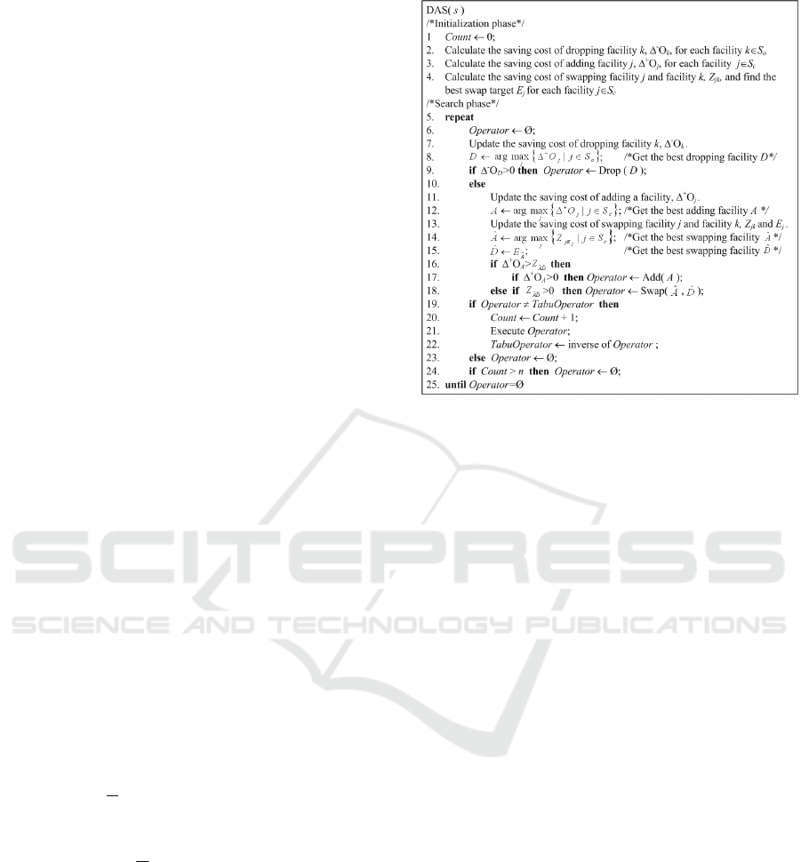
Figure 1: The DAS heuristic.

reduction of Swap(j, k), that is, opening j and closing

k, is denoted by equation (9).

The pseudo code for the Drop-Add-Swap

heuristic (DAS) is shown in Figure 1. In the pseudo

code, Drop(D) denotes closing facility D, Add(A)

denotes opening facility A, and Swap(A, D) denotes

opening facility A and closing facility D

simultaneously. As for the Multistart Drop-Add-

Swap heuristic (MDAS), it will randomly generate a

set of initial solutions first, and then it will apply the

DAS heuristic to each initial solution to search for

the optimum or near-optimal solution.

We now explain the DAS heuristic depicted in

Figure 1. Given a solution s, for each open facility k,

the saving cost of closing facility k will be

calculated; for each closed facility j, the saving cost

of opening facility j will be calculated; for each

closed facility j, the saving cost of opening facility j

and closing its best swapping target E

will also be

calculated (lines 2-4). After the initialization phase,

begins the search phase. The search phase contains

at most n iterations and in each iteration, at most one

of the three operations (Drop, Add and Swap) will

be applied. The algorithm terminates if the number

of iterations is greater than n or the chosen operation

is tabued or none of the three operations can reduce

the total cost. In each iteration, the Drop operation is

considered first. If the Drop operation can reduce the

total cost, the Drop operation that reduces cost most

will be applied (lines 7-9). Otherwise, the Add

operation and the Swap operation will be considered

simultaneously. Whichever of the Add operation and

the Swap operation can reduce the total cost most

THE MULTISTART DROP-ADD-SWAP HEURISTIC FOR THE UNCAPACITATED FACILITY LOCATION

PROBLEM

will be applied (lines 11-18). The inverse operation

of the applied operation will be tabued in the next

iteration (line 22). When applying any of Drop,

Add or Swap operation, from equations (5)-(9), it is

noted that only related information needs to be

updated rather than all information needs to be

recomputed. Therefore, the calculation of the net

cost change of an operation is very time efficient.

Moreover, by properly combining Drop, Add and

Swap operations, the MDAS heuristic is very

effective in solving the UFLP.

3 EXPERIMENTAL RESULTS

AND DISCUSSIONS

Extensive experiments had been conducted to

evaluate the performance of the proposed MDAS

heuristic. A personal computer with Intel Core 2

Duo 2.33 GHz CPU was used as the platform to run

the program. Although there were two processors,

only one processor was used. The program was

implemented using C++. In this section,

experimental results are given and some discussions

are made.

3.1 Benchmarks

Most benchmarks collected in the UflLib (Hoefer,

2002) website had been utilized to test the

performance of the MDAS heuristic. These

benchmarks are listed as follows.

ORLIB: This benchmark was proposed by (Beasley,

1993) and posted in OR-Library. It consists of 15

problems that are divided into four classes.

M*: These problems were presented by (Kratica et

al., 2001). The benchmark contains six sets with

problem size 100, 200, 300, 500, 1000 and 2000

respectively. Each set has five problems.

GR: The benchmark was proposed by (Galvao and

Raggi, 1989). It consists of five sets with problem

size 50, 70, 100, 150 and 200 respectively. Each set

contains ten problems.

BK: This benchmark, presented by (Bilde and

Krarup, 1977), contains 220 problems with size from

30×30 to 100×100. The distances between customers

and facilities are drawn uniformly from [0, 1000].

FPP: This benchmark was artificially generated to

make the problems harder to be solved. It was

proposed by (Kochetov and Ivanenko, 2003) at the

5th Metaheuristics International Conference in 2003.

The benchmark contains 40 problems and these

problems are classified into two classes: FPP11

(with m = 133 and n = 11) and FPP17 (with m = 307

and n = 17).

GAP: This benchmark was also proposed by

(Kochetov and Ivanenko, 2003) at the 5th

Metaheuristics International Conference. It consists

of three classes: GAPA, GAPB and GAPC. Each

class contains 30 problems. Since these problems

have larger duality gaps, they are more difficult to

be solved by the dual-base method.

GHOSH: (Ghosh, 2003) presented this benchmark

in 2003. The benchmark contains 90 problems.

These problems are divided into two classes:

symmetric and asymmetric. Each class is further

divided into three sets with problem size 250, 500

and 750 respectively. The optimal solutions of some

of these problems are still unknown.

MED: Originally, this benchmark was proposed by

(Ahn et al., 1998) as a benchmark for the p-median

problem. In 1999, (Barahona and Chudak, 1999)

modified it to act as a benchmark for the UFLP. This

benchmark consists of 18 problems with size 500,

1000, 1500, 2000, 2500 and 3000 respectively. For

each size, there are three problems with the opening

costs of facilities being set to

10n

100n

and

1000n

, respectively.

3.2 Performance comparison of MDAS

Heuristic and DROP Method

The comparison of performance of the DROP

method, the DAS heuristic and the MDAS heuristic

is shown in Table 1. The first column of Table 1

represents the problem name, the second column

represents the size of the problem, where m is the

number of customers and n is the number of

facilities. The third column lists the costs of the

optimal solutions. The fourth and the fifth column

list the deviation from the optimal solution of the

solution found by the DROP method and the DAS

heuristic, respectively, with the initial solution in

which all facilities were open.

The sixth column represents the average deviation

(from the optimal solutions) of the solutions found

by applying the MDAS heuristic ten times. In each

time, ten randomly generated solutions were used as

the initial solutions. The seventh column shows the

number of times by which the optimal solution was

found by the MDAS heuristic. Finally, the last

column denotes the average CPU time used by the

MDAS heuristic over ten times.

ICINCO 2009 - 6th International Conference on Informatics in Control, Automation and Robotics

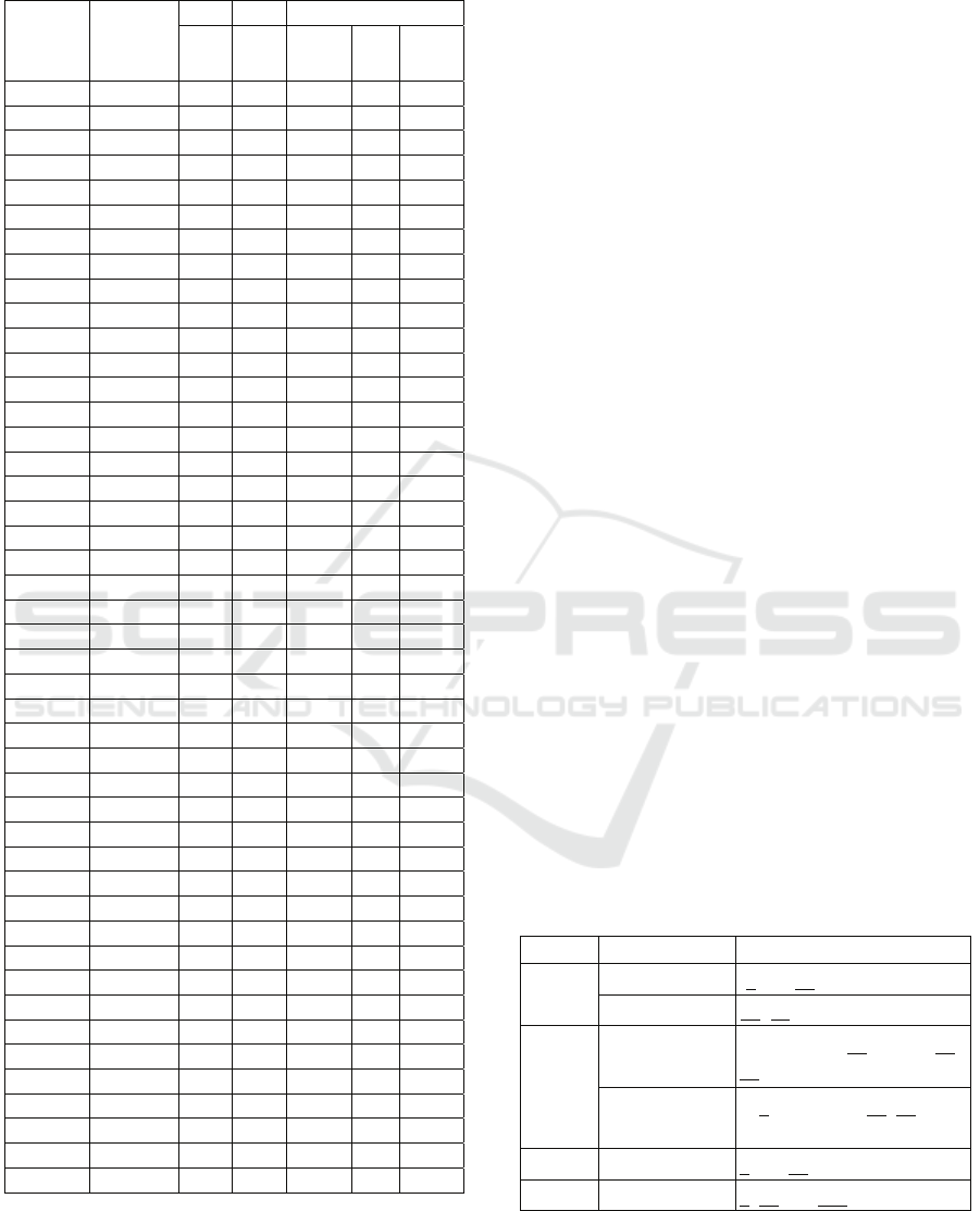
Table 1: Performance comparison of the DROP method,

the DAS heuristic and the multistart DAS heuristic.

Problem OPT

Dro

DAS MDAS

Dev Dev

AVG

Dev

Hit

AVG

Time

71 932615.75 0.00 0.00 0.00 10 0.000

72 977799.40 0.00 0.00 0.00 10 0.000

73 1010641.4 0.00 0.00 0.00 10 0.000

74 1034976.9 0.26 0.00 0.00 10 0.000

101 796648.44 0.00 0.00 0.00 10 0.000

102 854704.20 0.09 0.00 0.00 10 0.000

103 893782.11 0.00 0.00 0.00 10 0.000

104 928941.75 0.61 0.00 0.00 10 0.000

131 793439.56 0.00 0.00 0.00 10 0.000

132 851495.32 0.09 0.00 0.00 10 0.000

133 893076.71 0.08 0.08 0.00 10 0.000

134 928941.75 0.61 0.00 0.00 10 0.000

A 17156454. 6.95 0.00 0.00 10 0.084

B 12979071. 1.04 0.00 0.00 10 0.100

C 11505594. 1.24 0.26 0.00 10 0.109

MO1 1156.91 0.53 0.00 0.00 10 0.09

MO2 1227.67 0.00 0.00 0.00 10 0.08

MO3 1286.37 0.94 0.14 0.00 10 0.09

MO4 1177.88 0.16 0.00 0.00 10 0.09

MO5 1147.60 0.00 0.00 0.00 10 0.08

MP1 2460.10 0.00 0.00 0.00 10 0.041

MP2 2419.32 0.00 0.00 0.00 10 0.042

MP3 2498.15 0.00 0.00 0.00 10 0.042

MP4 2633.56 0.45 0.00 0.00 10 0.044

MP5 2290.16 0.00 0.00 0.00 10 0.044

1 3591.27 0.00 0.00 0.00 10 0.109

2 3543.66 0.04 0.00 0.00 10 0.109

3 3476.81 0.85 0.00 0.00 10 0.120

4 3742.47 0.00 0.00 0.00 10 0.111

5 3751.33 0.00 0.00 0.00 10 0.113

MR1 2349.86 0.00 0.00 0.00 10 0.362

MR2 2344.76 0.00 0.00 0.00 10 0.414

MR3 2183.24 0.00 0.00 0.00 10 0.400

MR4 2433.11 0.00 0.00 0.00 10 0.377

MR5 2344.35 0.00 0.00 0.00 10 0.372

MS1 4378.63 0.00 0.00 0.00 10 2.489

MS2 4658.35 0.05 0.00 0.00 10 2.586

MS3 4659.16 0.67 0.00 0.00 10 2.858

MS4 4536.00 0.00 0.00 0.00 10 2.427

MS5 4888.91 0.00 0.00 0.00 10 2.172

MT1 9176.51 0.00 0.00 0.00 10 14.986

MT2 9618.85 0.00 0.00 0.00 10 13.878

MT3 8781.11 0.00 0.00 0.00 10 14.654

MT4 9225.49 0.00 0.00 0.00 10 14.855

MT5 9540.67 0.00 0.00 0.00 10 13.775

From Table 1, it is noted that there are 17

problems on which the DROP method cannot find

optimal solutions, but there are only 3 problems on

which the DAS heuristic cannot find optimal

solutions. Hence, the DAS heuristic is superior to

the DROP method. Furthermore, when ten randomly

generated solutions were used as the initial solutions

instead of using only the solution with all facilities

opened, the MDAS heuristic could find optimal

solutions for all these 45 problems and for all ten

times of experiments.

Therefore, the MDAS heuristic enhances the

global search ability of the DAS heuristic and

improves the performance significantly. By

examining the solutions of the seventeen problems

on which the DROP method could not find optimal

solutions, some of the solutions were very close to

the optimal solutions, but the optimal solutions

could not be reached from these solutions by

applying the Drop operation. The three problems on

which the DAS heuristic could not find optimal

solutions had a similar situation. The solutions found

by the DAS heuristic for these three problems and

the optimal solutions of these three problems are

listed in Table 2. It is noted that two swap operations

(Swap(6, 11) and Swap(25, 15)) executed

simultaneously are needed to transform the solution

found by the DAS heuristic to the optimal solution

for Cap133. Similarly, more than two operations

executed simultaneously are needed to transform the

solutions found by the DAS heuristic to the optimal

solutions for the other two problems. But when the

DAS heuristic started with multiple randomly

generated initial solutions, though still being

restricted to executed only one operation in each

iteration, the multi-start DAS (MDAS) could find all

optimal solutions of all these forty-five problems as

shown in Table 1.

Table 2: The optimal solutions and the solutions found by

the DAS heuristic (all open).

Instance Source Solution

Cap133

OPT 6

, 23, 25, 27, 34, 45, 46, 49

DAS(All Open) 11, 15, 23, 27, 34, 45, 46, 49

Capc

OPT

6, 14, 24, 35, 53, 70, 79, 81,

DAS(All Open)

6, 9

, 14, 24, 35, 48, 66, 70,

MO3 OPT 6, 39, 48

DAS(All Open) 7, 38, 39, 100

THE MULTISTART DROP-ADD-SWAP HEURISTIC FOR THE UNCAPACITATED FACILITY LOCATION

PROBLEM

Table 3: Performance comparison of the MDAS heuristic with two other methods on six benchmarks.

3.3 Performance Comparison of

MDAS and the Other Two Methods

In this subsection, the performance of the MDAS is

compared with those of the hybrid multistart

heuristic and the simple tabu search on six

benchmarks. This comparison is depicted in Table 3.

The performance data of the hybrid multistart

heuristic and the simple tabu search were taken from

(Resende and Werneck, 2006). The six benchmarks

considered are ORLIB, M*, GR, BK, FPP and GAP.

The computer used by the MDAS was a personal

computer with Intel core2 Duo 2.33GHz CPU (only

one processor was used).

The computer used by the other two methods was

the SGI challenge with 28 196-MHz MIPS R10000

CPU (only one processor was used). In this

experiment, the MDAS was run 50 times on each

problem and the average was taken. In Table 3,

AvgD (in %) is defined as follows: AvgD=[(best

solution found by the method - best known upper

bound)/best known upper bound]*100.

Where the best known upper bound is taken from

(Hoefer, 2002). AvgT (in seconds) denotes the

average CPU time. It is noted that with just 10 seeds

(i.e., 10 randomly generated initial solutions), the

MDAS can find all the best solutions in all 50 times

(i.e., AvgD=0) on ORLIB, M* and GR benchmarks.

Also, the CPU time needed is much less than those

needed by the other two methods. For BK and FPP

benchmarks, the MDAS can also find all the best

solutions in all 50 times with 100 and 16000 seeds,

respectively. In solving these two benchmarks, the

CPU time need by the MDAS is also much less than

those needed by the other two methods. As for the

benchmark GAP, the MDAS found the best solution

of each problem in this benchmark within the 50

times of execution, but it could not find all best

solutions in any single time of execution. From

Table 3, it is observed that the MDAS outperforms

the other two methods in both the solution quality

and the computation time.

3.4 Performance Comparison of

MDAS and the other Three

Methods

In this subsection, the performance of the MDAS is

compared with those of Ghosh’s method (Ghosh,

1999), the hybrid multistart heuristic (Resende and

Werneck, 2006), and Sun’s tabu search (Sun, 2006)

on the GHOSH benchmark. There are totally 90

problems in this benchmark that are divided

according to size and type into 18 sets with five

problems in each set. The performance comparison

is shown in Table 4, within which the previous best

known solutions are taken from (Sun, 2006). Both

the data of the hybrid multistart heuristic and the

data of our MDAS are the average of 50 runs. It is

noted in Table 4 that Ghosh’s method achieves one

(out of eighteen) previous best known solution, the

hybrid multistart heuristic achieves four (out of

eighteen) previous best solutions, Sun’s tabu search

achieves fourteen (out of eighteen) previous best

solutions, and our MDAS achieves thirteen (out of

eighteen) previous best known solutions. Moreover,

the MDAS found solutions of the other four sets that

are better than the previous best known solutions

(the italics solutions in Table 4). The last row of

Class Method

ORLIB M* GR BK FPP GAP

Avg D Time Avg D Time Avg D Time Avg D Time Avg D Time Avg D Time

Hybrid

Iteration=8, Elite=5 0.000 0.05 0.004 2.19 0.000 0.09 0.028 0.09 69.370 1.63 9.573 0.348

Iteration=32, Elite=10 0.000 0.17 0.000 7.86 0.000 0.32 0.002 0.28 33.375 7.66 5.953 1.64

Iteration=2048, Elite=80 －－－－－－－－ 0.000 330.9 0.820 92.09

Simple

Tabu

500 Non-improving 0.028 0.16 0.011 1.75 0.100 0.16 0.071 0.16 95.711 0.65 15.901 0.26

64000 Non-improving －－－－－－－－ 71.150 52.08 6.350 22.43

MDAS

10 Random See

0.000 0.02 0.000 0.92 0.000 0.02 0.032 0.00 46.948 0.04 13.783 0.01

50 Random See

－－－－－－ 0.001 0.02 3.963 0.21 8.661 0.03

100 Random See

－－－－－－ 0.000 0.03 0.298 0.43 7.063 0.07

1000 Random See

－－－－－－－－ 0.012 4.46 2.930 0.74

4000 Random See

－－－－－－－－ 0.003 17.53 1.217 3.42

16000 Random See

－－－－－－－－ 0.000 67.36 0.559 20.30

ICINCO 2009 - 6th International Conference on Informatics in Control, Automation and Robotics

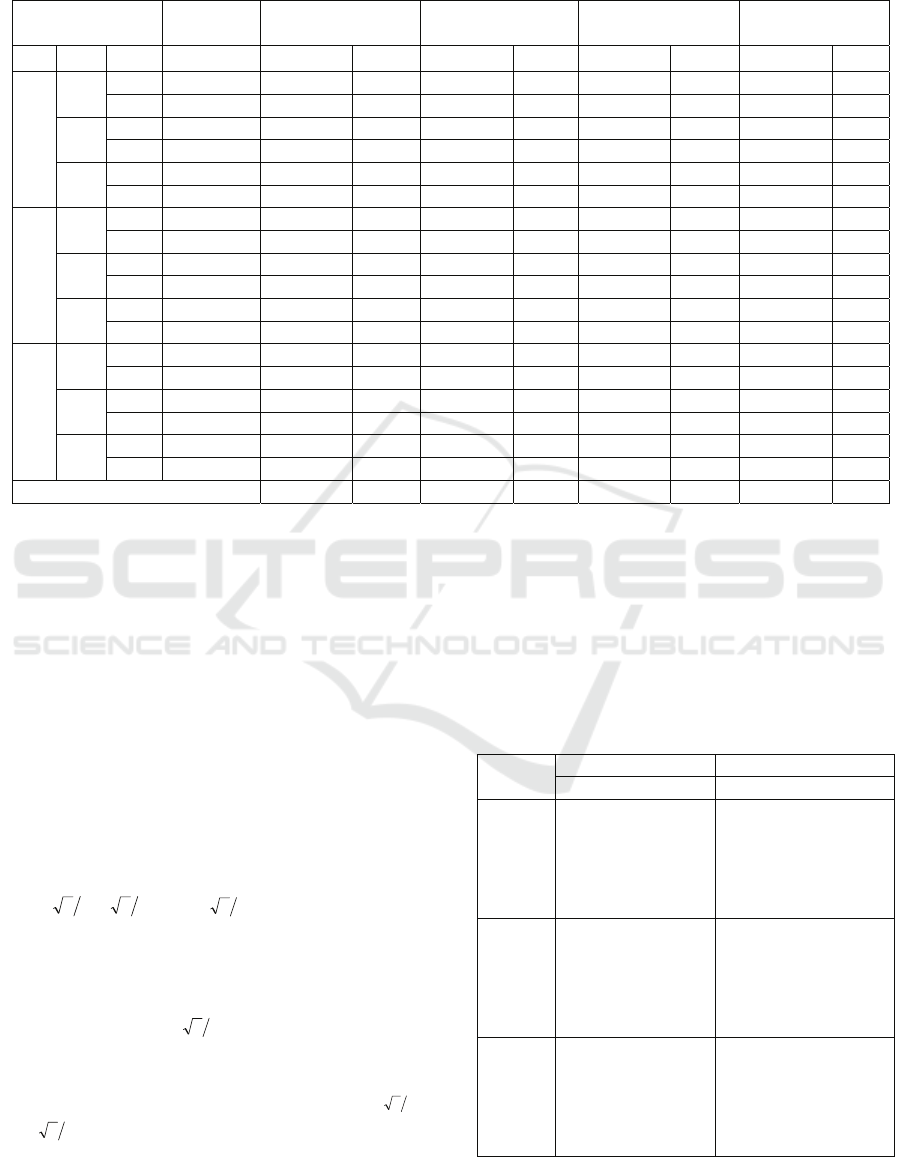
Table 4: Performance comparison of the MDAS heuristic and three other methods on benchmark GHOSH.

Instance

Previous best

known

Ghost Hybrid Tabu Search MDAS(1000Seed)

Class Size Type Value Best Time Best Time Best Time Best Time

250

257805.0 257832.6 18.256 257807.9 5.3 257805.0 2.828 257804.0 7.36

Asy

257917.8 257978.4 18.060 257922.1 5.7 257917.8 2.618 257917.8 7.32

500

511180.4 511383.6 213.316 511203.0 43.5 511180.4 15.616 511181.2 35.87

Asy

511140.0 511251.6 207.070 511147.4 40.3 511140.0 13.760 511136.4 35.97

750

763693.4 763831.2 824.288 763713.9 112.6 763693.4 39.812 763684.8 93.68

Asy

763717.0 763840.4 843.206 763741.0 117.5 763717.0 39.650 763716.4 92.60

250

276035.2 276185.2 6.470 276035.2 8.0 276035.2 5.628 276035.2 5.88

Asy

276053.2 276184.2 6.402 276053.6 8.2 276053.2 5.790 276053.2 5.92

500

537912.0 538480.4 71.394 537919.1 52.6 537912.0 31.432 537912.0 26.72

Asy

537847.6 538144.0 79.192 537868.2 52.2 537847.6 34.748 537847.6 26.73

750

796571.8 796919.0 409.372 796593.7 126.3 796571.8 93.352 796571.8 68.83

Asy

796374.4 796754.2 395.958 796393.5 127.1 796374.4 95.430 796374.4 64.71

250

333671.6 333671.6 17.322 333671.6 8.3 333671.6 9.878 333671.6 5.73

Asy

332897.2 333058.4 24.730 332897.2 7.4 332897.2 9.196 332897.2 5.67

500

621059.2 621107.2 146.482 621059.2 50.8 621059.2 71.106 621059.2 24.18

Asy

621463.8 621881.8 134.76 621475.2 57.4 621463.8 72.064 621463.8 26.60

750

900158.6 900785.2 347.414 900183.8 130.3 900158.6 229.914 900158.6 56.31

Asy

900193.2 900349.8 499.738 900198.6 136.5 900193.2 236.902 900193.2 56.95

Average 555535.489 236.847 555493.567 60.556 555316.189 56.096 555315.500 34.730

Table 4 lists the average values over the eighteen

sets, and from the average values, it is noted that the

MDAS outperforms the other three methods.

3.5 Performance Comparison of

MDAS and Hybrid Multistart

Heuristic on MED

The performance of the MDAS is compared with

that of the hybrid multistart heuristic on the

benchmark MED, and this comparison is shown in

Table 5. The MED benchmark contains 18 problems

with size 500, 1000, 1500, 2000, 2500 and 3000,

respectively. For each size n, there are three

problems with the opening costs of facilities being

set to

10n

100n

, and

1000n

, respectively.

In this experiment, the MDAS heuristic was run

50 times with 1000 seeds. It is noted in Table 5 that

the MDAS heuristic outperforms the hybrid

multistart heuristic on the first group in which the

facility’s open cost is

10n

. But the solution quality

of the hybrid multistart heuristic is better than that of

the MDAS heuristic on the second and the third

groups in which the facility’s open costs are

100n

and

1000n

, but the computation time of the latter is

less than that of the former.

Observing the above mentioned experimental

results, we conclude the following:

(1) The DAS heuristic that utilizes the Drop

operation, the Add operation and the Swap

operation performs better than the DROP

method that utilizes only the Drop operation.

Table 5: Performance comparison of the MDAS heuristic

with the hybrid multistart heuristic on benchmark MED.

instance

Hybri

MDAS(1000Seed)

Avg Time Avg Time

500-10 798577.0 33.2 798577.0 28.0

1000-10 1434185.4 173.9 1434171.0 130.7

1500-10 2001121.7 347.8 2000854.14 331.1

2000-10 2558120.8 717.5 2558121.5 687.4

2500-10 3100224.7 1419.5 3100174.5 1116.7

3000-10 3570818.8 1621.1 3570820.75 1667.0

500-100 326805.4 32.9 326922.375 25.6

1000-100 607880.4 148.8 607992.563 106.5

1500-100 866493.2 378.7 867149.688 293.6

2000-100 1122861.9 650.8 1123936.5 562.3

2500-100 1347577.6 1128.2 1348713.25 870.5

3000-100 1602530.9 1977.6 1605083.63 1349.5

500-1000 99196.0 23.6 99196.0 22.4

1000- 220560.9 141.7 220626.563 84.4

1500- 334973.2 387.2 335400.813 218.7

2000- 437690.7 760 438263.0 425.9

2500- 534426.6 1309.4 535134.938 675.3

3000- 643541.8 2081.4 644376.25 1017.3

THE MULTISTART DROP-ADD-SWAP HEURISTIC FOR THE UNCAPACITATED FACILITY LOCATION

PROBLEM

(2) The MDAS heuristic enhances the global

search capability of the DAS heuristic and the

performance of the MDAS heuristic will be

improved as the number of seeds increases.

(3) Although the MDAS heuristic is just a

heuristic, its performance is better than some state-

of-the-art metaheuristics. (Table 3 and 4)

The fact that the hybrid multistart heuristic

outperforms the MDAS heuristic on the second and

the third groups of the MED benchmark (Table 5)

indicates that the global search ability of the MDAS

heuristic is still not good enough for searching a

large solution space.

4 CONCLUSIONS

In this paper, the DAS heuristic and the multistart

DAS (MDAS) heuristic are proposed to solve the

UFLP. The DAS heuristic utilizes three operations:

the Drop operation, the Add operation, and the Swap

operation. And the MDAS heuristic enhances the

global search capability of the DAS heuristic by

applying it multiple times with different initial

solutions (seeds). Experimental results reveal that

the MDAS heuristic outperforms other state-of-the-

art heuristics on most of the benchmarks. But the

global search ability of the MDAS heuristic is still

not good enough for searching a large solution

space, therefore, in future studies, we will try to

combine a global search scheme with the DAS

heuristic to improve the performance. Also, we plan

to investigate the possibility of applying the

proposed heuristic to other combinatorial problems.

REFERENCES

Ahn, S., Cooper, C., Cornuéjols, G., Frieze, A.M., 1998.

Probabilistic analysis of a relaxation for the k-median

problem. Mathematics of Operations Research, (13) 1-

31.

Arya, V., Garg, N., Khandekar, R., Meyerson, A., 2001.

Munagala K, Pandit V. Local Search heuristics for k-

median and facility location problems. ACM

Symposium on Theory of Computing, 21-29.

Barahona, F., Chudak, F., 1999. Near-optimal solutions to

large scale facility location problems. Technical

Report RC21606, IBM, Yorktown Heights, NY, USA.

Beasley, J.E., 1993. Lagrangean heuristics for location

problems. European Journal of Operational Research,

(65) 383-399.

Bilde, O., Krarup, J., 1977. Sharp lower bounds and

efficient algorithms for the simple plant location

problem. Annals of Discrete Mathematics, (1) 79-97.

Cornuéjols, G., Nemhauser, G.L., Wolsey, L.A., 1990.

The uncapacitated facility location problem. in: P.B.

Mirchandani, R.L. Francis (Eds.), Discrete Location

Theory, Wiley-Interscience, New York, 119-171.

Erlenkotter, D., 1978. A dual-based procedure for

uncapacitated facility location. Operations Research,

(26) 992-1009.

Galvao, R.D., Raggi, L.A., 1989. A method for solving to

optimality uncapacitated facility location problems.

Annals of Operations Research, (18) 225-244.

Ghosh, D., 2003. Neighborhood search heuristics for the

uncapacitated facility location problem. European

Journal of Operational Research, (150) 150-162.

Hoefer, M., 2002. Performance of heuristic and

approximation algorithms for the uncapacitated

facility location problem. Research Report MPI-I-

2002-1-005, Max-Planck-Institutfür Informatik.

Hoefer, M., 2002. UflLib, http://www.mpi-

sb.mpg.de/units/agl/projects/benhmarks/UflLib.

Jain, K., Mahdian, M., Saberi, A., 2002. A new greedy

approach for facility location problems, in:

Proceedings of the 34th Annual ACM Symposium on

Theory of Computing (STOC), ACM Press, 731-740.

Kochetov, Y., Ivanenko, D., 2003. Computationally

difficult instances for the uncapacitated facility

location problem. in: Proceedings of the 5th

Metaheuristics International Conference (MIC), 41:1-

41:6.

Körkel, M., 1989. On the exact solution of large-scale

simple plant location problems, European Journal of

Operational Research, (39) 157-173.

Kratica, J., Tosic, D., Fillipovic, V., Ljubic, I., 2001

Solving the simple plant location problem by genetic

algorithm. RAIRO Operations Research, (35) 127-

142.

Kuehn, A.A., Hamburger, M.J., 1963 A heuristic program

for locating warehouses. Management Science (9)

643-666.

Mahdian, M., Ye, Y., Zhang, J., 2002. Improved

approximation algorithms for metric facility location

problems, in: Proceedings of the 5th International

Workshop on Approximation Algorithms for

Combinatorial Optimization (APPROX), volume 2462

of Lecture Notes in Computer Science, Springer-

Verlag, 229-242.

Michel, L., Van Hentenryck, P., 2003. A simple tabu

search for warehouse locatiohn. European Journal of

Operational Research, (157) 576-591.

Nemhauser, G.L., Wolsey, L.A., Fisher, L.M., 1978 An

analysis of approximations for maximizing

submodular set functions, I. Mathematical

Programming, (14) 265-94.

Resende, M.G.C., Werneck, R.F., 2006. A hybrid

multistart heuristic for the uncapacitated facility

location problem. European Journal of Operational

Research, (174) 54-68.

Sun, M., 2006. Solving the uncapacitated facility location

problem using tabu search. Computers & Operations

Research, (33) 2563-2589.

ICINCO 2009 - 6th International Conference on Informatics in Control, Automation and Robotics