ANALOG REALIZATIONS OF FRACTIONAL-ORDER

INTEGRATORS/DIFFERENTIATORS

A Comparison

Guido Maione

DEESD, Technical University of Bari, Via de Gasperi, snc, I-74100, Taranto, Italy

Keywords: Non-integer-order operators, Fractional-order controllers, Rational approximation, Interlaced singularities.

Abstract: Non-integer differential or integral operators can be used to realize fractional-order controllers, which

provide better performance than conventional PID controllers, especially if controlled plants are of non-

integer-order. In many cases, fractional-order controllers are more flexible than PID and ensure robustness

for high gain variations. This paper compares three different approaches to approximate fractional-order

differentiators or integrators. Each approximation realizes a rational transfer function characterized by a

sequence of interlaced minimum-phase zeros and stable poles. The frequency-domain comparison shows

that best approximations have nearly the same zero-pole locations, even if they are obtained starting from

different points of view.

1 INTRODUCTION

Originally, the investigation of integrals and

derivatives of any order was a topic known as

fractional calculus. In recent years, however,

considerable attention has been paid to the concept

of non-integer derivative and integral to model

systems in various fields of science and engineering.

In the research area of control theory, several

authors have provided generalizations of classical

controllers introducing various types of Fractional-

Order Controllers (FOC). For example, the CRONE

(French acronym for “Commande Robuste d’Ordre

Non Entièr”) controller (Oustaloup, 1991;

Oustaloup, 1995) and Fractional-Order Proportional-

Integral-Derivative (FOPID) controllers PI

(Podlubny, 1999a; Podlubny, 1999b) have been

recently considered. Moreover, FOC have been

successfully applied in rigid robots, both for position

control and for hybrid position-force-control

(Tenreiro Machado and Azenha, 1998; Valerio and

Sá da Costa, 2003). In general, FOC provide better

performance than PID controllers, if the controlled

plants are of non-integer-order. In other cases, FOC

show high flexibility and can ensure high robustness

for high gain variations. More particularly, in SISO

systems, they can make the phase margin nearly not

changing in a wide range around the gain crossover

frequency, even if high gain variations produce high

changes in gain crossover frequency. Applications in

mechatronics are testified by several papers (Canat

and Faucher, 2005; Li and Hori, 2007; Ma and Hori,

2004a; Ma and Hori, 2004b; Ma and Hori, 2007;

Melchior et al., 2005).

The basic element of transfer functions of

FOPID controllers is the fractional

differentiator/integrator s

, with ν positive or

negative real number. This operator is infinite

dimensional, even if it can be approximated by

finite-dimension transfer functions, whose

coefficients depend on the non-integer exponent ν. A

good rational approximation can be obtained by

truncating the continued fractions expansion (CFE)

of s

(Maione, 2006; Maione, 2008). Recently, in

(Barbosa et al., 2006), least-squares-based methods

are used for obtaining Fractional-Order Differential

Filters (FODF) approximating s

In this paper, a novel approach is compared to

two commonly used methods to realize a rational

approximation of fractional-order differentiators or

integrators. These operators are the basic elements in

fractional-order controllers of mechatronic systems.

Section 2 revisits the three different methods

systematically. Section 3 compares them in the

frequency domain. Section 4 draws the conclusion

with some remarks.

184

Maione G.

ANALOG REALIZATIONS OF FRACTIONAL-ORDER INTEGRATORS/DIFFERENTIATORS - A Comparison.

DOI: 10.5220/0002173901840189

In Proceedings of the 6th International Conference on Informatics in Control, Automation and Robotics (ICINCO 2009), page

ISBN: 978-989-674-001-6

2 REVISITING THREE

RATIONAL APPROXIMATIONS

In this section, three methods are compared. They

are shortly revisited, for making a direct comparison

based on transfer functions putted in the same form.

All the considered realizations are known to be

minimum-phase and stable, with poles interlacing

zeros along the negative real half-axis of the s-plane.

This property is enlightened by the form of the three

transfer functions, which explicitly shows the

frequencies corresponding to the alternated zeros

and poles. The interlacing property is important for

comparison purposes, because the position of the

zero-pole pairs determines the quality of the models

approximating phase and magnitude of the irrational

operator (jω)

. Hence, for comparison purpose,

realizations are constrained to have both their zeros

with minimum module and their poles with

maximum module approximately equal. All the

approximating transfer functions are in a factorized

form, which puts in evidence the break frequencies.

Then, the lowest and highest break frequencies of

the proposed method are taken as reference.

2.1 The Proposed CFE Approximation

The starting point is the following continued

fractions expansion (CFE):

()

 1

+++

+≅+

(1)

with b

= b

= 1, a

= ν x and:

= n (n–ν) x, b

= 2n (2)

= n (n+ν) x, b

= 2n+1 (3)

for j = 2n, with n natural number (Khovanskii,

1965). The analog approximation for the operator s

with 0 < ν < 1, is given in (Maione, 2008), where

x = s–1 is used in (1) to obtain the (2N)-th

convergent of the resulting CFE as approximating

transfer functions:

)( )( )(

),(

ννν

qsqsq

pspsp

+++

−



(4)

where

(ν) = q

N,N-j

(ν) =

= (–1)

C(N, j) (ν+j+1)

(

)

(ν– N)

(

)

(5)

and

)!(!

),(

jNj

jNC

−

is the binomial

coefficient. Moreover:

(ν+j+1)

(

)

= (ν+j+1) (ν+j+2) … (ν+N) (6)

(ν–N)

(

)

= (ν–N) (ν–N+1) … (ν–N+j+1) (7)

define the Pochammer functions with (ν–N)

(0)

= 1

(Spanier and Oldham, 1987). As it is easily noted, in

this method the coefficients p

(ν) and q

(ν) are

explicitly given in terms of the fractional order ν.

Obviously, the positions of zeros and poles in the s-

plane also depend on ν. So,

),(

can be written

in the form:

∏

≅

ksG

),(

(8)

As it is proved in (Maione, 2008), zeros

)

(

−

and poles

)

(

−

of ),(

are all real and

interlace along the negative real half-axis in the

s-plane, with:

pzpzpz

2211

 .

(9)

2.2 Oustaloup’s Recursive

Approximation

The CRONE controller is an integer-order frequency

domain approximation of s

in the form:

∏

≅

ksG

),(

(10)

The gain k is adjusted so that G(ν,s) has the same

crossover frequency as the ideal operator s

. The

number N of zeros and poles of the approximating

transfer function is chosen in advance. They

alternate on the negative real half-axis of the s-plane

so that the frequencies satisfy:

pzpzpz



2211

(11)

ANALOG REALIZATIONS OF FRACTIONAL-ORDER INTEGRATORS/DIFFERENTIATORS - A Comparison

185

In this way, zeros and poles interlace on the

negative real half-axis, leading to a gain which is,

approximately, a linear function of the logarithm of

frequency. The phase is nearly constant and

approximates ν π / 2. The parameters ω

and ω

are

determined by placing zeros and poles as follows:

ηωω

νν

⎟

⎠

⎞

⎜

⎝

⎛

⎟

⎠

⎞

⎜

⎝

⎛

−

; ;

(12)

= i = 1, ..., N

(13)

1 ii

i = 1, ..., N–1.

(14)

The frequencies

and ω

are appropriately

chosen as

< and

> , so that it holds

≅ and

≅ .

2.3 Matsuda’s Approximation

The Matsuda’s method approximates the operator s

from its gain

. The gain is determined at 2N+1

frequencies

, ω

, …, ω

, which are taken

logarithmically spaced in the approximation interval.

The interval [

, ω

] is chosen so that the lowest

break frequency

and the highest break

frequency

in the model satisfy:

≅ and

≅

, respectively. Note that, usually, an odd

value of

N is used, so that the resulting

approximation is proper. Then, the following

functions are defined:

)()(

)(

;

)()(

)( ;

;

)()(

)( ;)(

121212

111

000

−−−

−

−−−

−

NNN

kkk

ωω

ωωω

……

…

(15)

from which the following set of parameters are

obtained:

()

ωα

(16)

)()(

111

−−−

−

kkkk

ωω

(17)

for

k = 1, 2, …, 2N.

Using the

and α

, the CFE can be written as:



−

+≅

sss

(18)

whose convergents provide the rational

approximations to the irrational operator s

. The

N)-th convergent of (18) can be easily converted

into the rational approximation, as the ratio

),(

of two polynomials with degree

N. Then, the

factorization of these polynomials leads to:

∏

≅

ksG

),(

(19)

Numerical experiments show that, also in this

case, it holds:

pzpzpz

ˆˆˆˆˆˆ

2211

 .

(20)

3 A COMPARISON BETWEEN

THREE METHODS

The approaches of the previous sections are here

compared, by choosing

N = 3 and then N = 4. These

values are chosen to make the order of the FOC

realizations as low as possible, compatibly with

good performances. Figures 1, 2, 3 and 4 show the

Bode plots of phase and amplitude, for the typical

fractional order

ν = 0.5. Other values of the integer

N and of ν, with 0 < ν < 1, can be considered. As

previously stated, the approximation is performed so

that

),(

, G(ν,s) and ),(

have their first

zero-frequency and their last pole-frequency nearly

equal. Hence, the zero-frequency

and the pole-

frequency

of ),(

are assumed as

reference. In conclusion, it must nearly hold:

≅

≅ , and

≅

when

N = 3, and

≅

≅ ,

≅

and

≅

, when N = 4.

First, the parameters of

),(

are determined.

For

ν = 0.5 and N = 3, formula (8) gives:

0.0521 =

, 0.6360 =

, 4.3119

ICINCO 2009 - 6th International Conference on Informatics in Control, Automation and Robotics

186

0.2319 =

, 1.5724 =

, 19.1957

, and

0.1429

=k . These values clearly indicate that

),(

is minimum-phase, stable, with interlacing

zeros and poles. Figure 1 reports the phase Bode

diagram of

)],(

[

ων

jGarg (Maione’s curve).

-2

-1

Frequency (rad/s)

Phase (degrees)

Ideal

Oustaloup

Matsuda

Maione

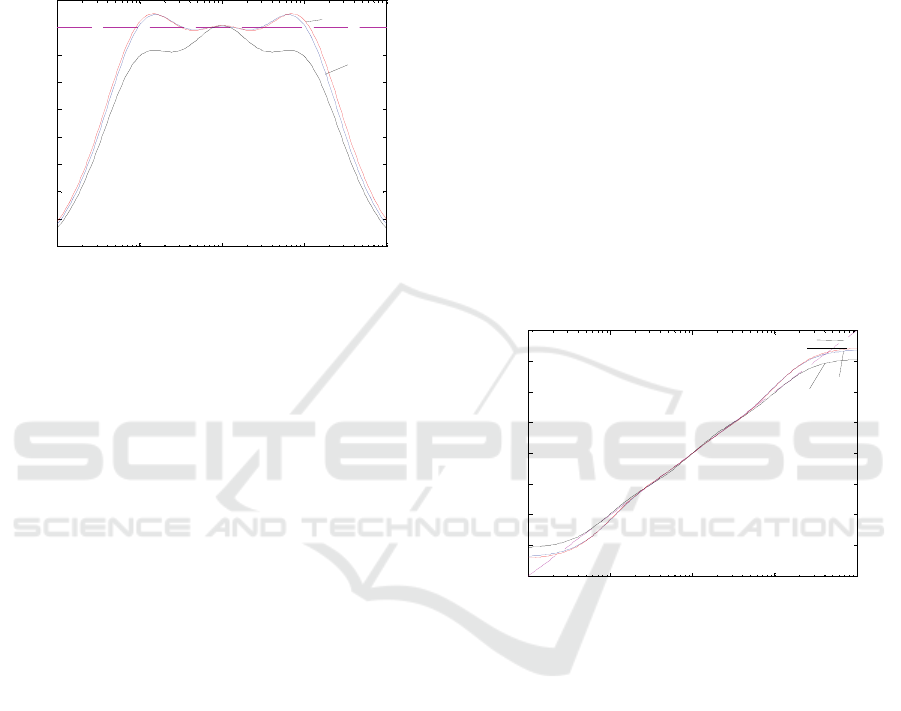
Figure 1: Phase Bode diagram for the approximations of

order 3 a fractional-order differentiator, ν = 0.5.

Now, the procedure for determining the function

G(ν,s) is considered. With reference to (12), the

interval [

, ω

] is chosen larger than ]

[

More precisely,

= and

where

and λ

are coefficients to be fixed so that

the Oustaloup’s algorithm leads to

≅ and

≅ . These coefficients are chosen by a rule

of thumb. Since

0521.0

and

1957.19

simple computer experiments in MATLAB

show

that choosing

= 0.55 and λ

= 1.8 yields:

0518.0

, 5509.0

, 8634.5

1688.0

, 7972.1

, 1293.19

, k =

0.1692. As it is noted, the constraints

≅

and

≅ are respected. In Figure 1, arg[G(ν, jω)]

is also reported (Oustaloup’s curve).

Finally, for applying the Matsuda’s method, the

sampling frequencies are logarithmically distributed

inside the approximation interval, so that it must

result:

≅ and

≅

, as requested. This

result is achieved by choosing

2 zN

= and

0 p

= . The parameter λ is fixed by computer

experiments to

λ = 45. Namely, the following

breaking frequencies of

),(

ων

jG result:

0.0485 =

, 0.6248 =

, 4.5311 =

0.2207 =

, 1.6004 =

, 0.6273 2=

, and

0.1373=

k . These values show that the constraints

≅

and

≅

are also satisfied. As it

can be easily observed, however, all the remaining

frequencies and the gain of the Matsuda’s model are

nearly equal to those of the author’s approximating

transfer function. This fact is confirmed by the

behaviour of

)],(

[

ων

jGarg in Figure 1 (Matsuda’s

curve). The Bode plot, indeed, is nearly

indistinguishable from the plot of

)],(

[

ων

jGarg .

In conclusion, Figure 1 shows that

)],(

[

ων

jGarg and )],(

[

ων

jGarg are nearly flat

and give a good approximation of

2 / ])[(

πνω

=jarg

. The plot of )],(

[

ων

jGarg

yields a slightly worst approximation. Figure 2

confirms that the magnitude plots of

),(

and

),(

are nearly coincident. They give a better

approximation of

than G(ν,s), also in this case.

-2

-1

-20

-15

-10

-5

Frequency (rad/s)

Amplitude (dB)

Maione

Oustaloup

Mats uda

Ideal

Figure 2: Amplitude Bode diagram for the approximations

of order 3 of a fractional-order differentiator, ν = 0.5.

Now, let us consider a different approximation

obtained by using

N = 4 and the same procedure.

For

ν = 0.5, formula (8) gives: 0.0311 =

0.3333 =

, 1.4203

, 7.5486

0.1325 =

0.7041 =

3.0000

32.1634

, and 0.1111

=k . Then, ),(

minimum-phase, stable, with interlacing zeros and

poles. Figure 3 shows the phase Bode diagram of

)],(

[

ων

jGarg (Maione’s curve).

For the Oustaloup’s approximation,

= 0.61 and

= 1.64 yield: 0311.0

, 2261.0

6419.1

, 9237.11

0839.0

6093.0

, 4247.4

, 1323.32

, and

k = 0.1377. The constraints

≅ and

ANALOG REALIZATIONS OF FRACTIONAL-ORDER INTEGRATORS/DIFFERENTIATORS - A Comparison

187

≅ are respected. In Figure 3, arg[G(ν, jω)]

is also reported (Oustaloup’s curve).

For the Matsuda’s approximation,

λ = 39 gives:

0.0310 =

, 0.3327 =

, 1.4211 =

7.5702 =

, 0.1321 =

, 0.7035 =

3.0055=

, 32.2772=

, and 0.1109=

k .

For

N = 4, the frequency response of )],(

[

ων

jGarg

is practically indistinguishable from that of

)],(

[

ων

jGarg

(Matsuda’s and Maione’s curves are

practically the same).

-2

-1

Frequency (rad/s)

Phase (degrees)

Ideal

Maione

Matsuda

Oustaloup

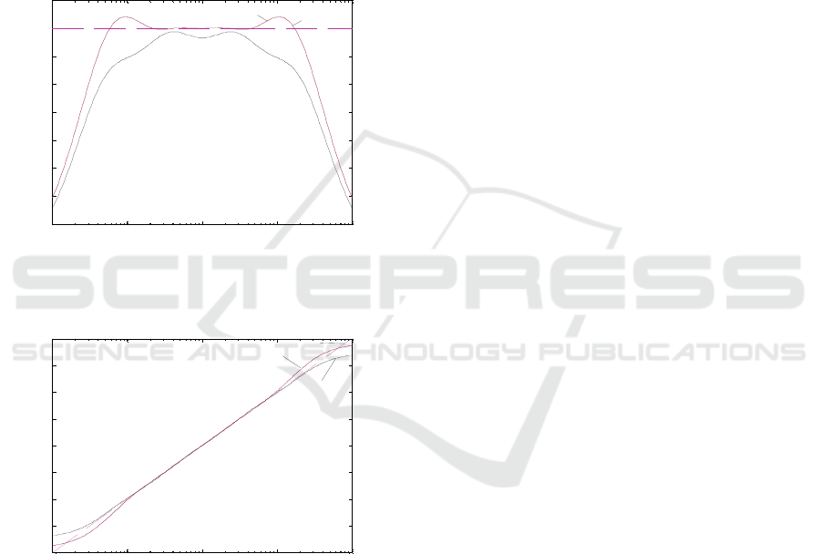
Figure 3: Phase Bode diagram for the approximations of

order 4 of a fractional-order differentiator, ν = 0.5.

-2

-1

-20

-15

-10

-5

Frequency (rad/s)

Amplitude (dB)

Ideal

Maione

Matsuda

Oustaloup

Figure 4: Amplitude Bode diagram for the approximations

of order 4 of a fractional-order differentiator, ν = 0.5.

Figure 4 confirms that the magnitude plots of

),(

and ),(

are nearly the same and give a

better approximation of

than G(ν,s), for N = 4.

4 CONCLUDING REMARKS

This paper compared three different methods to

approximate non-integer-order differential or

integral operators in fractional-order controllers:

these methods are the author’s, the Oustaloup’s, and

the Matsuda’s, respectively. All approximations of

the irrational operator

were realized through

analog transfer functions characterized by stable

poles and minimum-phase zeros. In particular, zeros

and poles were interlaced along the negative real

half-axis of the

s-plane, and the first and last

singularities were constrained to be nearly the same

in all approximations. The interlacing property

allowed us the comparison to find the best

distribution of singularities. Namely, a frequency

domain analysis of the phase diagrams showed that

the author’s and Matsuda’s approximations

outperformed the well-known by Oustaloup.

Note that all realizations were limited to the

lowest order that could guarantee good performance.

The better results achieved by the proposed

approximation are due to a better distribution of

interlaced zeros and poles. It is also interesting to

note how the proposed approximation achieves

nearly the same zero-pole pairs of the Matsuda’s

approximation, even if the starting points of the two

methods are completely different.

REFERENCES

Barbosa, R.S., Tenreiro Machado, J.A., Silva, M.F., 2006.

Time domain design of fractional differintegrators

using least-squares. Signal Processing, Vol. 86, No.

10, pp. 2567-2581.

Canat, S., Faucher, J., 2005. Modeling, identification and

simulation of induction machine with fractional

derivative. In Fractional Differentiation and its

Applications, Le Mehauté, A., Tenreiro Machado,

J.A., Trigeassou, J.C., Sabatier, J. (Eds.), Ubooks

Verlag Ed., Neusäß, Vol. 2, pp. 195-206.

Khovanskii, A.N., 1965. Continued fractions. In

Lyusternik, L.A., Yanpol’skii, A.R. (Eds.):

Mathematical Analysis - Functions, Limits, Series,

Continued Fractions, chap. V, Pergamon Press.

Oxford, International Series Monographs in Pure and

Applied Mathematics (transl. by D. E. Brown).

Li, W., Hori, Y., 2007. Vibration suppression using single

neuron-based PI fuzzy controller and fractional-order

disturbance observer. IEEE Transactions on Industrial

Electronics, Vol. 54, No. 1, pp. 117-126.

Ma, C., Hori, Y., 2004a. Backlash vibration suppression

control of torsional system by novel fractional-order

PID

controller. Transactions of IEE Japan on

Industry Application, Vol. 124, No. 3, pp. 312-317.

Ma, C., Hori, Y., 2004b. Fractional order control and its

application of PI

D controller for robust two-inertia

speed control. In Proceedings of the 4th International

Power Electronics and Motion Control Conference

ICINCO 2009 - 6th International Conference on Informatics in Control, Automation and Robotics

188

(IPEMC 04), Xi'an, China, 14-16 Aug. 2004, Vol. 3,

pp. 1477-1482.

Ma, C., Hori, Y., 2007. Fractional-order control: theory

and applications in motion control (past and present).

IEEE Industrial Electronics Magazine, Winter 2007,

Vol. 1, No. 4, pp. 6-16.

Maione, G., 2006. Concerning continued fractions

representation of noninteger order digital

differentiators. IEEE Signal Processing Letters, Vol.

13, No. 12, pp. 725-728.

Maione, G., 2008. Continued fractions approximation of

the impulse response of fractional order dynamic

systems. IET Control Theory & Applications, Vol. 2,

No. 7, pp. 564-572.

Melchior, P., Sabatier, J., Duboy, D., Ferragne, H.,

Amagat, C., 2005. CRONE position controller for

pneumatic butterfly valve controller by on-off valves.

In Fractional Differentiation and its Applications, Le

Mehauté, A., Tenreiro Machado, J.A., Trigeassou,

J.C., Sabatier, J. (Eds.), Ubooks Verlag Ed., Neusäß,

Vol. 3, Chap. 16, pp. 721-734.

Oustaloup, A., 1991. La Commande CRONE. Commande

Robuste d’Ordre Non Entièr, Editions Hermès. Paris,

France.

Oustaloup, A., 1995. La Dérivation non Entière: Théorie,

Synthèse et Applycations, Editions Hermès, Serie

Automatique. Paris, France.

Podlubny, I., 1999a. Fractional Differential Equations,

Academic Press. San Diego, CA, USA.

Podlubny, I., 1999b. Fractional-order systems and PI

controllers. IEEE Transactions on Automatic Control,

Vol. 44, No. 1, pp. 208-214.

Spanier, J., Oldham, K.B., 1987. An atlas of functions,

Hemisphere Publishing Co.. New York, 1987.

Tenreiro Machado, J.A., Azenha, A., 1998. Fractional-

order hybrid control of robot manipulators. In IEEE

SMC’98, Proceedings of the 1998 IEEE International

Conference on Systems, Man, and Cybernetics, Hyatt

La Jolla, San Diego (CA), USA, 11-14 Oct. 1998, pp.

788-793.

Valerio D., Sá da Costa, J., 2003. Digital implementation

of non-integer control and its application to a two link

control arm. In Proceedings of the European Control

Conference, Cambridge, UK, 1-4 Sept. 2003.

ANALOG REALIZATIONS OF FRACTIONAL-ORDER INTEGRATORS/DIFFERENTIATORS - A Comparison

189