
VARIABLE GEOMETRY TRACKED UNMANNED GROUNDED
VEHICLE
Model, Stability and Experiments
Jean-Luc Paillat, Phillipe Lucidarme and Laurent Hardouin
Laboratoire d’Ing
´
enierie des Syst
`
emes Automatis
´
es (LISA), 62 Avenue Notre Dame du Lac, Angers, France
Keywords:
UGV (Unmanned ground vehicle), Variable Geometry Single Tracked Vehicle (VGSTV), Obstacle clearing
capabilities, Teleoperation, Stability, Geometric model, Dynamic model.
Abstract:
This paper introduces an originally designed tracked robot. This robot belongs to the VGSTV (Variable
Geometry Single Tracked Vehicle) category. It is equipped with two tracks mounted on an actuated chassis.
The first joint is used to articulate the chassis and the second one to keep the tracks tightened. By controlling
the chassis joint it becomes possible to adapt the shape of the tracks to the ground and even to release the
tracks in order to pass through specific obstacles. A prototype has been build ; technical specifications and
dynamic model are presented in this paper. Tele-operated experiments have been conducted and have shown
that the stability of the robot have to be addressed. We experimented and compared two classical criterions
based on the center of mass and on the zero moment point technique. Experimental results are discussed in
the case of a staircase clearing.
1 INTRODUCTION
UNMANNED GROUNDED VEHICLE (UGV) is a
topically research field applied to a wide range of ap-
plications like for example exploration or missions
in hostile environments. Research laboratories and
robotics companies are currently working on the de-
sign of tele-operated and autonomous robots. Accord-
ing to (Casper and Murphy, 2003) and (Carlson and
Murphy, 2005) UGVs can be classified into three cat-
egories :
• Man-packable delineates the robots that can be
carried by one man in backpacks.
• Man-portable delineates the robots that are too
heavy to be easily carried by men, but small
enough to be transported in a car or a HUMMV.
• Not man-portable delineates the robots that must
be carried by a truck, a trailer or a crane.
The robots presented in this paper are classified
in the man-packable and man-portable categories. In
this class of robots, designers have to face the follow-
ing dilemma: on one hand, build a small robot that
can be easily carried and move into narrow environ-
ments. Unfortunately, it will generally result in poor
obstacle clearing capability. On the other hand, build
a bigger robot will increase its ability to surmount ob-
stacles but will not enable the robot to go through nar-
row openings. The challenge is then to build a robot
as small as possible with the higher obstacle clear-
ing capability. Based on this observation the first part
of this paper introduces the existing experimental and
commercial robots and discusses about their clearing
capabilities. The following of the paper describes
an originally designed UGV (Fig. 2b). This robot
can be classified into the Variable Geometry Single
Tracked Vehicle (VGSTV) category, i.e. it has the
mechanical ability to modify its own shape according
to the ground configuration. The design of our proto-
type is described in the third part with a short discus-
sion about the technical choices (information can be
found on the project website: http://www.istia.univ-
angers.fr/LISA/B2P2/b2p2.html). The next section
introduces the dynamic model of the robot. The first
tele-operated experiments have shown that the mass
distribution is crucial to pass through large obstacles.
This is why the last section discusses about the sta-
bility of the robot. The presented survey has been
conducted for three reasons. First of all, the informa-
tion computed about the stability of the robot may be
useful to the operator during tricky operations. Sec-
ondly, this information may also be used to automati-
cally disable clumsy commands and prevent the robot
21
Paillat J., Lucidarme P. and Hardouin L. (2009).
VARIABLE GEOMETRY TRACKED UNMANNED GROUNDED VEHICLE - Model, Stability and Experiments.
In Proceedings of the 6th International Conference on Informatics in Control, Automation and Robotics - Robotics and Automation, pages 21-28
DOI: 10.5220/0002182000210028
Copyright
c
SciTePress
from toppling over. And finally, the stability cannot
be ignored during autonomous motion which is our
long term goal. The survey has been conducted on
two criterions : static (the center of mass) and dy-
namic (based on the well known zero moment point
technique). Experimental results are compared and
discussed in the case of a staircase clearing. A gen-
eral conclusion ends the paper.
2 EXISTING UGVs
2.1 Wheeled and Tracked Vehicles with
Fixed Shape
This category gathers non variable geometry robots.
Theoretically, this kind of vehicles are able to climb a
maximum step twice less high than their wheel diam-
eter. Therefore their dimensions are quite important
to ensure a large clearing capability. This concep-
tion probably presents a high reliability (Carlson and
Murphy, 2003) but those robots cannot be easily used
in unstructured environments like after an earthquake
(Casper and Murphy, 2003).
Figure 1: a) Talon-Hazmat robot (Manufacturer: Foster-
Miller) b)ATRV-Jr robot. Photo Courtesy of AASS,
¨
Orebro
University.
2.2 Variable Geometry Vehicle
A solution to ensure a large clearing capability and to
reduce the dimensions consists in developing tracked
vehicles which are able to modify their geometry in
order to move their center of mass and climb higher
obstacles than their wheel’s diameters.
Figure 2: a)Packbot (manufacturer: IRobot), b)RobuROC
6(Manufacturer: Robosoft) c)Helios VII.
The Packbot robot (Fig. 2a) is probably one of the
most famous commercial VGTV (Variable Geometry
Tracked Vehicle). This robot is equipped with tracks
and two actuated tracked flippers (372 mm long). The
flippers are used to step over the obstacles. The obsta-
cle clearing capability of this kind of VGTV depends
on the size of the flippers. For more information and a
detailed survey on clearance capability of the Packbot
the reader can consult (Frost et al., 2002).
The robuROC6 (Fig. 2b) is equipped with 46.8
cm diameters wheels and can clear steps until 25cm
(more than half the diameter of the wheels). Joints
between the axles make this performance possible.
An other original system called Helios VII (Fig 2c)
(Guarnieri et al., 2004) is equipped with an arm ended
by a passive wheel which is able to elevate the chassis
along a curb.
2.3 Variable Geometry Single Tracked
Robots
Actually, there is a subgroup in VGTV called Variable
Geometry Single-Tracked Vehicles (VGSTV) (Kyun
et al., 2005). It gathers robots equiped with as tracks
as propulsion motors. In most cases those robots are
equipped with one or two tracks (one for each side).
It can be divided into two groups :
• robots with deformable tracks,
• robots with non deformable tracks.
2.3.1 Non-deformable Tracks VGSTV
Figure 3: a) Micro VGTV (manufacturer: Inuktun Ltd)
b)B2P2 prototype c)VGSTV mechanism.
The most famous example is the Micro VGTV. Il-
lustrations of a prototypes manufactured by the com-
pany Inuktun are presented on Fig. 3a. This robot
is based on an actuated chassis used to modify the
shape of the robot. The right picture of Fig. 3a shows
the superimposing configurations. The tracks are kept
tightened by a passive mechanism. The robot is thus
equipped with three motors: two for the propulsion
and one for the chassis joint.
Non commercial vehicles exists in the literature
as the VGSTV mechanism (Fig. 3c) which is ded-
icated to staircase clearing. It is composed of two
tracks and two articulations which allow it to have
many symmetrical configurations such as a rectangle,
ICINCO 2009 - 6th International Conference on Informatics in Control, Automation and Robotics
22
trapezoids, inverse trapezoids etc.
Many other VGTV architecture exist, for further
information reader can consult (Vincent and Tren-
tini, 2007), (Misawa, 1997), (Clement and Villedieu,
1987), (Guarnieri et al., 2004) and (Kyun et al., 2005).
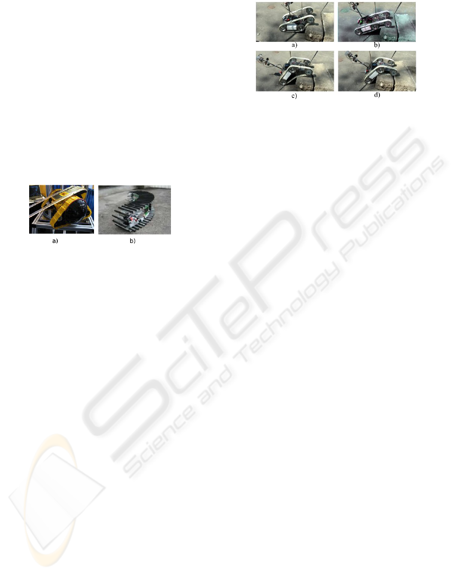
2.3.2 Deformable Tracks VGSTV
Some single tracked robots have the ability to modify
the flexing of their tracks. Two examples presented
on Fig. 4, are able to adapt their shape to obstacles
(Kinugasa et al., 2008). However, even if the control
of the robot seems easier with a flexible track than
with a non flexible one, the mechanical conception
could be more complicated.
Figure 4: a) Viper robot (Manufacturer: Galileo) b)Rescue
mobile track WORMY.
According to the presented state of the art, for gen-
eral purpose missions we beleive that the best com-
promise between design complexity, reliability, cost
and clearing capabilities is the Variable geometry sin-
gle tracked robots category. The next section will in-
troduce and describe our prototype of VGSTV.
3 PROTOTYPE DESCRIPTION
The main interest of VGSTV (equipped with de-
formable tracks or not) is that it is practicable to
overcome unexpected obstacles (Kyun et al., 2005).
Indeed, thanks to the elastic property of the tracks
the clearance of a rock in rough terrain will be more
smoothly with a VGSTV (e. g. Fig 3 and 4) than with
a VGTV (Fig. 2). On the Micro VGTV presented
on Fig. 3, the tension of the tracks is mechanically
linked with the chassis joint so it is constant during
the movement. Nevertheless, in some cases, less
tense tracks could increase the clearance capability
by increasing the adherence. An interesting study
about this point was developed by (Iwamoto and
Yamamoto, 1983) giving a VGSTV able to climb
staircases where the tension of the tracks was me-
chanically managed as on the MicroVGTV (Fig. 3a).
However, this system was equipped with a spring to
allow the tracks to adapt their shape to the ground
(depending on the strength of the spring).
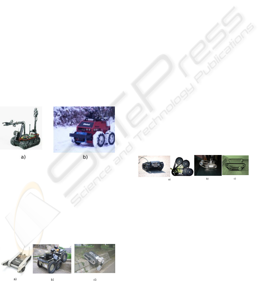
Figure 5: B2P2: clearing of a curb.
The conception of our prototype is based on this
previous work, but we decided to actuate the tension
of the tracks. Indeed, by using two motors instead
of one (Fig. 6) it is possible to increase the tracks
adaptation to the ground developed by (Iwamoto and
Yamamoto, 1983) and reach new configurations for
the robot. As example, the solution proposed in this
paper allows our robot to adopt classical postures of
VGSTV (Fig. 5(a), 5(b) and 5(c) ), but also other in-
teresting positions. On Fig. 5 B2P2 is clearing a curb
of 30 cm height with tense tracks. The position of the
robot on Fig 5(c) can also be obtained with the Mi-
cro VGTV, but it is a non-safety position and B2P2 is
close to topple over. On Fig. 5(d) the tracks have just
been released. They take the shape of the curb and it
can be cleared safely. This last configuration outlines
the interest of using an active system instead of a pas-
sive one. Consequently, although our prototype (Fig.
3b) belong to the VGSTV category and have not de-
formable tracks, it has the ability to adapt them to the
ground (as deformable ones).
Besides, even if there is a risk of the tracks coming
off, loosening the tracks may be an efficient mean of
increase the surface in contact with the floor in rough
terrain and then to improve the clearing capability of
the structure. By the way, the risk could decreased
by using sensor based systems to control the tension
of the tracks or by modifying the mechanical struc-
ture of the robot (adding some kind of cramps on the
tracks or using a guide to get back the tracks before it
comes off).
3.1 Mechanical Description
This UGV is equipped with four motors. Fig. 6
presents the integration of the motors in the robot.
Motors 1 and 2 are dedicated to the propulsion
(tracks).
The actuated front part is composed of motors 3
and 4 :
• Motor 3 actuates the rotational joint, it allows the
rotation of the front part around the second axle.
• Motor 4 actuates a driving screw, it controls the
VARIABLE GEOMETRY TRACKED UNMANNED GROUNDED VEHICLE - Model, Stability and Experiments
23
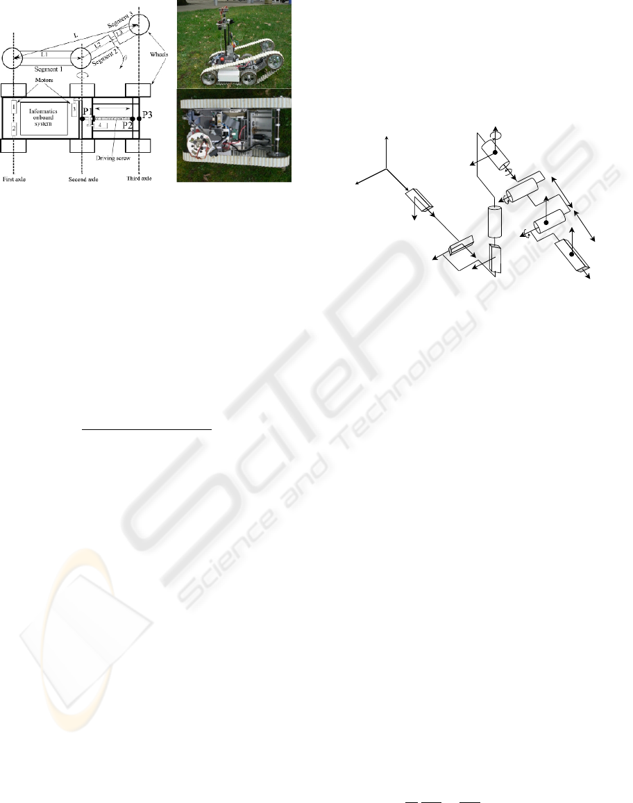
distance between the second axle and the third
one.
Figure 6: Overview of the mechanical structure, side and
top view of the real robot.
To keep the tension of the tracks the trajectory of
the third axle is given by an ellipse defined by two
seats located on the first and the second axle.
L + (L
2
+ L
3
) = K (1)
where the lengths L, L
2
and L
3
are referenced on
Fig. 6. K is a constant parameter depending on the
length of the tracks, L
3
evolves in order to achieve
equality (1) and is linked to the angle θ in the follow-
ing manner:
L
3
=
L
2
1
− K
2
2(L
1
cos(π− | θ |) − K)
− L
2
(2)
3.2 Sensors and Command Systems
The robot is equipped with multiple sensors, on-
board/command systems and wireless communica-
tion systems.
• Onboard command systems :
– PC104 equipped with a Linux OS compiled
specifically for the robot needs based on a LFS
(Home made light linux distribution).
– An home-made I2C/PC104 interface.
– Four integrated motor command systems run-
ning with RS232 serial ports.
– Four polymer batteries which allow more than
one hour of autonomy.
• Sensors :
– An analog camera for tele-operation.
– A GPS to locate the robot in outdoor environ-
ments.
– A compass to know the orientation of the robot.
– A two axis inclination sensor (roll and pitch).
• Wireless communication systems :
– A 2.4 GHz analog video transmitter.
– A bidirectional 152 MHz data transmitter.
4 DYNAMIC MODEL
3
4
5
O7
O8
Z4, X 5, Z1
Z5, X 6
X8
Z7
X7
Z8
O4, O5, O6
Z6
X4
X3
6
7
8
2
Z1
X2
Z2
X0
Y 0
Z0
O0
1
X1
L
1
L
2
+ L
3
Figure 7: B2P2’s geometric model. Joints 1,2 and 3 rep-
resents the robot position. Joints 4, 5 and 6 symbolize re-
spectively the yaw, roll and pitch, 7 and 8 are the actuated
joints.
This section deals with the dynamic model of the
robot which is based on the geometric model (Fig. 7)
detailed on (Paillat et al., 2008). According to this
model, the robot motion in a 3D frame (R
0
) is de-
scribed by the vector q of the 8 joints variables :
q = [q
1
,q
2
,q
3
,q
4
,q
5
,q
6
,q
7
,q
8
]
T
The dynamic model of a mechanical system es-
tablishes a relation between the effort applied on the
system and its coordinates, generalized speeds and ac-
celerations ((Craig, 1989) and (Khalil and Dombre,
2004)). In this section, the following notations are
used:
• j describes the joints from 1 to 8,
• i describes the segments from 1 to 3 (referenced
on Fig 6),
• n and m describes indexes from 1 to 8.
4.1 The Dynamic Equations
The general dynamic equations of a mechanical sys-
tem is:
d
dt
∂ L
∂ ˙q
j
−
∂ L
∂ q
j
= Q
j
+ T
j
(3)
ICINCO 2009 - 6th International Conference on Informatics in Control, Automation and Robotics
24

• L is the Lagrangien of the system. It is composed
of rigid segments, so there is no potential energy.
Although the Lagrangien corresponds to the ki-
netic energy.
• q
j
is the j
th
joint variable of the system.
• Q
j
is the gravity’s torque applied to the j
th
joint
of the system.
• T
j
is the external force’s torque applied to the j
th
joint of the system.
The kinetic energy is given by:
K =
n
∑
i=1
1
2
m
i
v
T
i
v
i
+
1
2
w
T
i
I
i
w
i
. (4)
• m
i
is the mass of the i
th
element of the model,
• v
i
is the linear speed of the i
th
element’s center of
gravity,
• w
i
is the angular speed of the i
th
element’s center
of gravity,
• I
i
is the matrix of inertia of the i
th
element of the
system.
In order to have homogeneous equations, w
i
is de-
fined in the same frame as I
i
; it allows to formulate v
i
and w
i
according to q :
v
i
= J
v
i
(q) ˙q (5)
w
i
= R
T
0 j
J
w
i
(q) ˙q (6)
where J
v
i
and J
w
i
are two matrices and R
0 j
is the
transport matrix between the frame R
0
and the frame
j linked to the segment i.
The kinetic energy formula is:
K =
1
2
˙q
T
∑
i
[m
i
J
v
i
(q)
T
J
v
i
(q) + J
T
w
i
(q)R
0 j
I
i
R
T
0 j
J
w
i
(q)] ˙q
(7)
which can be rewritten as :
K =
1
2
˙q
T
D(q) ˙q (8)
by developing the previous formula, we obtain :
K =
1
2
∑
m,n
d
m,n
(q) ˙q
m
˙q
n
(9)
where d
m,n
(q) is the m, n
th
element of the matrix D(q).
The gravity’s torque is given by:
Q
j
=
∑
i
gm
i
∂ G
0
zi
∂ q
j
. (10)
• G
0
zi
is the z coordinate of the CoG of the i
th
seg-
ment’s computed in the base frame (R
0
),
• g is the gravity acceleration.
Vector T (defined in (3)) is composed of the
external forces’ torque. For the robot presented here,
there is no consideration of external forces, so the T
vector only describes the motorized torques. Joints
1, 4, 7 and 8 are motorized, so the vector T is given
by those four parameters. T
1
and T
4
are computed
from the torques of motors 1 and 2 while T
7
and T
8
are deduced from motors 3 and 4.
The Euler-Lagrange equations can be written as:
∑
m
d
jm
(q) ¨q
m
+
∑
n,m
c
nm j
(q) ˙q
n
˙q
m
= Q
j
+ T
j
(11)
c
nm j
=
1
2
[
∂ d
jm
∂ q
n
+
∂ d
jn
∂ q
m
−
∂ d
nm
∂ q
j
] (12)
which is classically written as:
D(q) ¨q +C(q, ˙q) ˙q = Q + T (13)
where D(q) represents the matrix of inertia and
C(q, ˙q) the centrifuge-coriolis matrix where X
jm
, the
jm
th
element of this matrix, is defined as :
X
jm
=
∑
n
c
nm j
˙q
n
.
Finally, the J
vi
and J
wi
matrix considered in (5)
and (6) have to be computed.
4.2 J
vi
and J
wi
Matrix Formulation
The matrix which links articular speed and general
speed of a segment is computed from the linear and
angular speeds formulas. The goal is to find a matrix
for each segment. They are composed of 8 vectors
(one for each joint of the model).
The computation consists in formulating in the
base frame, the speed (V
P
i
( j − 1, j)
R
0
) of a point P
i
given by a motion of the joint q
j
attached to the frame
j according to the frame j − 1. Those parameters
can be deduced from the law of composition speeds
and the Denavitt Hartenberg (DH) formalism used for
the geometric model (Paillat et al., 2008). Indeed,
the general formulation is simplified by the geometric
model. Only one degree of freedom (DoF) links two
frames using the DH model and this DoF is a revolute
or a prismatic joint. Moreover, the Z axis is always the
rotation or translation axis, so the angular and linear
speeds are given by four cases:
• The angular speed of a point for a revolute joint:
VARIABLE GEOMETRY TRACKED UNMANNED GROUNDED VEHICLE - Model, Stability and Experiments
25

w
P
( j − 1, j)
R
0
= R
0, j
0
0
1
˙q
j
. (14)
• The linear speed of a point for a revolute joint:
v
P
( j − 1, j)
R
0
= V
R
j−1
O
j
+V
R
j
P
+ w
j
∧ O
j
P
R
j
= ˙q
j
R
0, j
0
0
1
∧ R
0, j
P
j
.
(15)
• The angular speed of a point for a prismatic joint:
w
P
( j − 1, j) =
0
0
0
. (16)
• The linear speed of a point for a prismatic joint:
v
P
( j − 1, j)
R
0
= R
0, j
0
0
1
˙q
j
(17)
where P
j
is the P point’s coordinates in R
j
.
Thus, the matrix of a segment i is formulated by com-
puting speeds for each joints as :
v
i
w
i
= J(q) ˙q = [J
1,i
(q),J
2,i
(q),...J
8,i
(q)] ˙q (18)
where J
j,i
(q) is a vector which links the speed of
the i
th
segment according to the j
th
joint. The first
segment is not affected by the motion of joints 7 and
8 while the second is not affected by joint 8, therefore
J
7,1
(q), J
8,1
(q) and J
8,2
(q) are represented by a null
vector.
5 BALANCE CRITERION
The balance criterion used here are the ZMP (Zero
Moment Point), widely used for the stability of hu-
manoid robots and the Center of Gravity (CoG). Pre-
vious theoretical works and experiments have proved
the ZMP efficiency (Vukobratovic and Borovac,
2004). It consists in keeping the point on the ground
at which the moment generated by the reaction forces
has no component around x and y axis ((Kim et al.,
2002) and (Kajita et al., 2003)) in the support poly-
gon of the robot. When the ZMP is at the border of
the support polygon the robot is teetering. Unlike the
ground projection of the center of gravity, it takes into
account the robot’s inertia.
The purpose of the following is to defined the co-
ordinates of this point in any frame of the model ac-
cording to the configuration of the robot. The defini-
tion can be implemented into the Newton equations
to obtain those coordinates. In any point of the model
: M
0
= M
z
+ OZ ∧ R (M
0
and M
z
define respectively
the moment generated by the reaction force R at the
points 0 and z).
According to the previous definition, there is no
moment generated by reaction forces at the Zero Mo-
ment Point. Consequently, if Z defines the ZMP co-
ordinates M
0
= OZ ∧ R. This formulation can be im-
plemented into the Newton equations as:
δ
0
= M
0
+
~
OG ∧
~
P +
~
OG ∧
~
F
i
(19)
where P is the gravity force, G is the robot’s center
of gravity and F
i
is the inertial force (the first New-
ton’s law gives F
i
= −m
¨
G). According to the ZMP
definition, the equation (19) can be formulated as :
δ
0
=
~
OZ ∧
~
R +
~
OG ∧
~
P +
~
OG ∧
~
F
i
(20)
δ
0x
= Z
y
R
z
+ G
y
P
z
− G
z
P
y
− G
z
Fi
y
δ
0y
= −Z
x
R
z
+ G
z
P
x
− G
x
P
z
(21)
Z
y
=
δ
0x
−G
y
P
z
+G
z
P
y
+G
z
Fi
y
R
z
Z
x
=
−δ
0y
+G
z
P
x
−G
x
P
z
R
z
.
(22)
Also, it is possible to compute the position of the
ZMP as a function of q (δ
0
depends on the matrix
D(q)).
Assuming the ground knowledge, the ZMP com-
putation gives a criterion to determinate the stability
of the platform.
6 RESULTS
This section presents the numerical computation of
the criterion in the case of the clearance of a stair-
case (staircase set of 15 cm risers and 28 cm runs)
with an average speed of 0.13 m.s
−1
(Fig. 9). The
robot is equipped with a 2-axis inclination sensor that
provides rolling and pitching. Vector q entries are
measured using encoders on each actuated axis of the
robot. Data have been stored during the experiments
and the models (CoG and ZMP) have been computed
off-line. This computation does not take into account
the tracks’ weight which is negligible in regard to the
robot’s weight. Fig. 8 presents the evolution of the
ZMP (left) and the difference between those two cri-
terion (right) during all the clearance. P
1
P
2
and P
3
ICINCO 2009 - 6th International Conference on Informatics in Control, Automation and Robotics
26
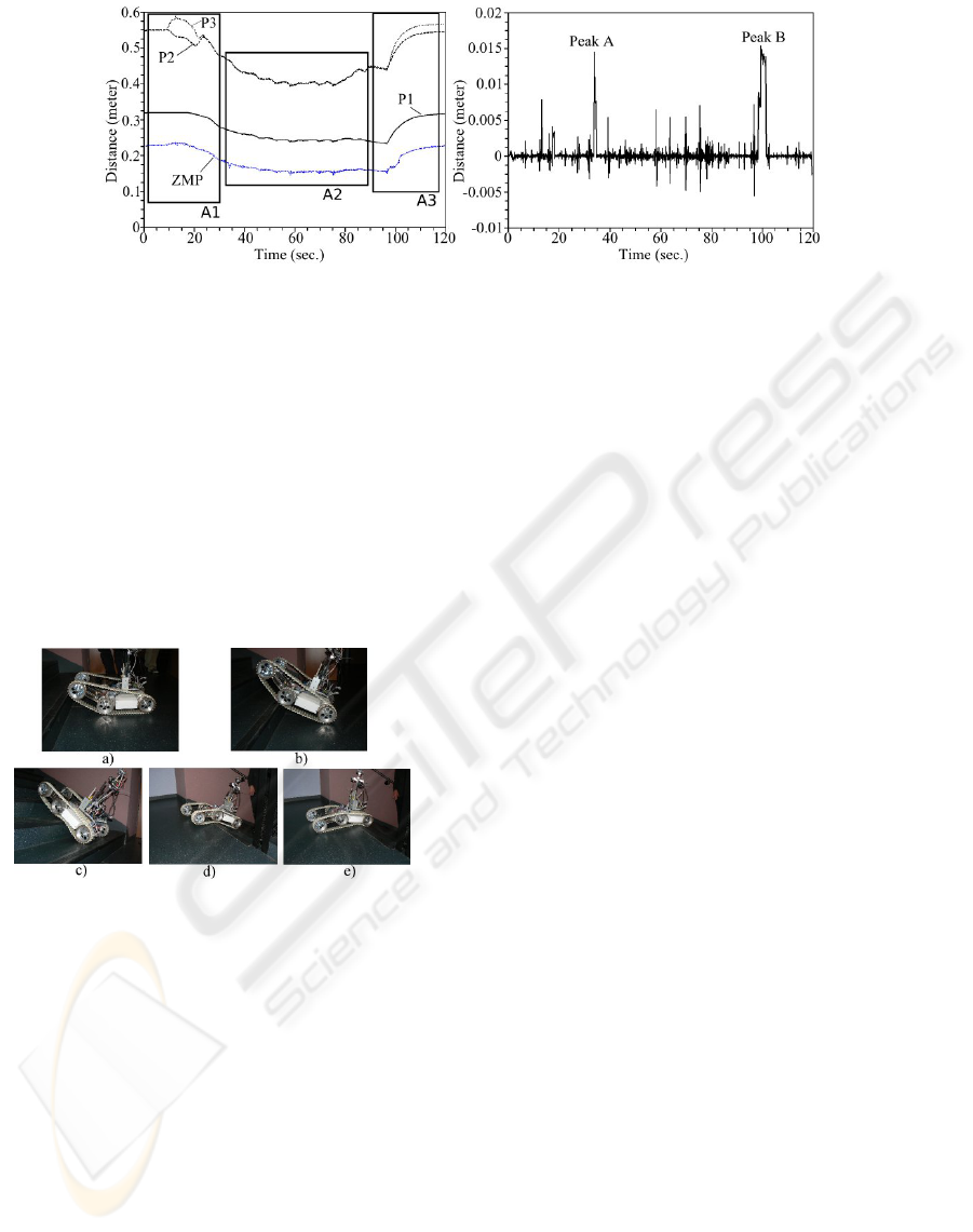
Figure 8: Experiment’s results. The left chart represents the evolution of the ZMP and the right one, the difference between
CoG and ZMP.
represents the z-coordinates in the frame R
5
(Fig. 7)
of three points of the robot which localization are no-
ticed on Fig. 6.
The following section finely details the results of
the experiment and the correlation with the sensors
data is described. This analyze is divided into three
parts: the approach of the first step, the clearance of
the middle steps and the clearance of the final step.
6.1 The Clearance of the First Step
Figure 9: Clearance of a staircase.
First of all, the robot is approaching while moving
up the front part (Fig. 9(a)) in order to go onto the first
step. Then, it has to move forward and move down
the elevation articulation in order to keep the stability
(Fig. 9(b)). Once the robot is step onto the first stair,
the operator have to switch in the next configuration.
The area noted A1 on Fig. 8 shows the evolution of the
ZMP projection during the clearance of the first step.
Note that the tracks are tense because when the front
part is rising up, there is a large difference between P
2
and P
3
.
6.2 The Clearance of the Middle Steps
This stage starts in the position noticed on Fig. 9(c).
By moving forward, the robot naturally climbs the
stairs. At each step, the robot is gently swaying when
the ZMP is passing over the step. This phenomenon
is illustrated by the oscillation of the ZMP which are
visible on the area noted A2 on Fig. 8. Note that, this
oscillation is dependent on the ratio between the size
of the robot and the size of the steps (”size-step” ra-
tio). It fully disappears when the length of the robot
is superior to the size of three steps. On the other
hand, oscillations may be more important until reach-
ing a ”size-step” ratio where the robot cannot climb
the step.
6.3 The Clearance of the Final Step
The robot is moving forward while moving down its
front part (Fig. 9(d)). This operation brings the ZMP
closer to the limits of the support polygon, i.e. the
corner of the last step. This operation allows a smooth
swing of the ZMP. Area A3 on Fig. 8 shows the evo-
lution of the ZMP during the clearing of the last step.
Note that the tracks releasing was not used dur-
ing this experiment because it was not necessary to
overcome this staircase. It could become essential for
bigger obstacles.
This experiment allows us to validate the pre-
sented model and confirms the computation of the
ZMP criterion. However, as it is shown on Fig. 8, the
average difference between the ZMP and the COG is
insignificant (about 0.21%). Moreover, the two peaks
(A and B) on the Fig. 8 are not due to the dynamics of
the system but to measurement errors. As the accel-
eration is measured with the encoders (linked to the
motor shaft), when the tracks slip, the measurement
is erroneous. The ZMP is computationally more ex-
pensive, needs more sensor measurements and the dif-
ference with the CoG is negligible. For these reasons,
we conclude that the CoG seems well suited for this
kind of experiments. Anyway, in the case where fast
obstacle clearance may be necessary, the CoG may
not longer be considered and the ZMP must be used
instead.
VARIABLE GEOMETRY TRACKED UNMANNED GROUNDED VEHICLE - Model, Stability and Experiments
27

7 CONCLUSIONS
In this paper, an original prototype of VGSTV has
been presented. The dynamic model have been intro-
duced. From this model, a stability criterion based on
the ZMP technique has been computed. This model
have been validated on the real robot in the context of
a staircase clearance.
Future works will focus on the autonomy of the
robot. In a short term work, a real time stability as-
sistance will be provided to the operator based on the
model (CoG or ZMP) presented in this paper. The
presented results are also a preliminary survey for
a long term work that will be oriented on the au-
tonomous obstacle clearance. Actual work (based on
the model and results presented here) is focused on
the automatic control of the robot.
REFERENCES
Carlson, J. and Murphy, R. R. (2003). Reliability analysis of
mobile robots. International Conferenee on Robotics
and Automation.
Carlson, J. and Murphy, R. R. (2005). How ugvs physi-
cally fail in the field. IEEE Transactions on robotics,
21(3):423–437.
Casper, J. and Murphy, R. R. (2003). Human-robot interac-
tions during the robot-assisted urban search and res-
cue response at the world trade center. IEEE Trans-
actions on systems, man, and cybernetics, 33(3):367–
384.
Clement, G. and Villedieu, E. (1987). Variable geometry
track vehicle. Us patent.
Craig, J. J. (1989). Introduction to Robotics Mechanics and
control. Silma, 2 edition.
Frost, T., Norman, C., Pratt, S., and Yamauchi, B. (2002).
Derived performance metrics and measurements com-
pared to field experience for the packbot. Proceedings
of the 2002 PerMIS Workshop.
Guarnieri, M., Debenest, P., Inoh, T., Fukushima, E., and
Hirose, S. (2004). Development of helios vii : an
arm-equipped tracked vehicle for search and rescue
operations. IEEE/RSJ Int. Conference on Intelligent
Robots.
Iwamoto, T. and Yamamoto, H. (1983). Variable configura-
tion track laying vehicle (us patent).
Kajita, S., Kanehiro, F., Kaneko, K., Fujiwara, K., Harada,
K., Yokoi, K., and Hirukawa, H. (2003). Biped walk-
ing pattern generation by using preview control of
zero moment point. Proceedings of the 2002 IEEE
Internationnal Conference on Robotics ans Automa-
tion.
Khalil, W. and Dombre, E. (2004). Modeling, Identification
and Control of Robots. Kogan Page Science, 2 edition.
Kim, J., Chung, W. K., Youm, Y., and Lee, B. H. (2002).
Real time zmp compensation method using null mo-
tion for mobile manipulators. Proceedings of the 2002
IEEE Internationnal Conference on Robotics ans Au-
tomation.
Kinugasa, T., Otani, Y., Haji, T., Yoshida, K., Osuka, K.,
and Amano, H. (2008). A proposal of flexible mono-
tread mobile track. Internationnal Conference on In-
telligent Robots and Systems.
Kyun, L. S., Il, P. D., Keun, K. Y., Byung-Soo, K.,
and Sang-Won, J. (2005). Variable geometry single-
tracked mechanism for a rescue robot. IEEE Inter-
national Workshop on Safety, Security and Rescue
Robotics, pages 111–115.
Misawa, R. (1997). Stair-climbing crawler transporter. Us
patent.
Paillat, J. L., Lucidarme, P., and Hardouin, L. (2008). Vari-
able geometry tracked vehicle, description, model and
behavior. Conference Mecatronics.
Vincent, I. and Trentini, M. (2007). Shape-shifting tracked
robotic vehicle for complex terrain navigation: Char-
acteristics and architecture. Technical memorandum,
Defence R and D Canada.
Vukobratovic, M. and Borovac, B. (2004). Zero-momment
point - thirty five years of its life. Internationnal jour-
nal of humanoid Robotics, 1(1):157–173.
ICINCO 2009 - 6th International Conference on Informatics in Control, Automation and Robotics
28
