A MIN-PLUS APPROACH FOR TRAFFIC FLOW MODELING
Julien Rousseau, S´ebastien Lahaye
LISA, 62 avenue Notre Dame du Lac, 49000 Angers, France
Claude Martinez
IRCCYN, 1 rue de la No¨e, 44000, Nantes, France
Jean-Louis Boimond
LISA, 62 avenue Notre Dame du Lac, 49000 Angers, France
Keywords:
Min-plus algebra, Min-plus linear systems, Vehicular traffic flow modeling, Traffic flow simulation.
Abstract:
In this paper we propose a modeling method for traffic flow phenomena based on the min-plus algebra. We
adopt a modular approach by dividing roadways as elementary stretches which can be combined in order
to get a model for a complex infrastructure. The approach is flexible in the sense that different scales can
be considered for each elementary model. In fact, whatever its size, each roadway stretch is here studied as
a min-plus linear system and is modeled by its impulse response in min-plus algebra. In this first step in
studying traffic flow, we focus on modeling detailing the adopted methodology. We also present simulations
to validate the approach.
1 INTRODUCTION
Traffic is a non-linear phenomenon complex to pre-
dict or simulate. In spite of that, many models for
traffic flow were studied since the late fifties, some at
a macroscopic level (for example models based on gas
kinetic, see (Helbing, 1996)), others at a microscopic
level (for example models based on cellular automata,
see (Nagel and Schreckenberg, 1992)).
In this paper we propose a modeling method for traf-
fic flow phenomena based on the min-plus algebra.
Previous works have used min-plus algebra to study
road traffic (Lolito et al., 2005), (Farhi et al., 2007).
In these papers, authors present a microscopic model
based on Petri nets whose dynamics are written using
min-plus algebra. This approach is not far from cel-
lular automata approach (Nagel and Schreckenberg,
1992) since roadways are divided in stretches contain-
ing at most one vehicle, and individual movement of
a vehicle in a stretch is conditioned by its availability
(no vehicle on this section).
The proposed approach is more flexible in the sense
that different scales can be considered for the model.
We also adopt a modular approach by dividing road-
ways as elementary stretches which can be combined
in order to get a model for a complex infrastructure.
But the scale of a stretch can be larger. In fact, what-
ever its size, each roadway stretch is here studied as
a min-plus linear system and is modeled by its im-
pulse response in min-plus algebra. In the extreme, a
stretch can be sized to contain a single vehicle. It can
also correspond to a more macroscopic element (e.g.
a roadway which is several kilometers long). Doing
so, we expect that descriptions of various phenomena
(inherent to various roadway configurations such as
intersections, traffic lights,...) can be modulated ac-
cording to their complexity and that large problems
can be tackled. Whereas analytical results were de-
rived in (Lolito et al., 2005), (Farhi et al., 2007), we
here focus on modeling of traffic flow. In fact, this
first paper aims only at stating the adopted modeling
methodology. We present simulations to validate the
approach.
The paper is organized as follows.
In section 2, we show that vehicular traffic flow can be
considered as a min-plus linear system, that is a linear
system over min-plus algebra. Representation of such
a system thanks to its impulse response is recalled.
159
Rousseau J., Lahaye S., Martinez C. and Boimond J. (2009).
A MIN-PLUS APPROACH FOR TRAFFIC FLOW MODELING.
In Proceedings of the 6th International Conference on Informatics in Control, Automation and Robotics - Intelligent Control Systems and Optimization,
pages 159-166
DOI: 10.5220/0002182301590166
Copyright
c
 SciTePress

In section 3, we propose a methodology to model traf-
fic flow as a min-plus linear system. A particular 2
inputs-2 outputs system is presented as a generic rep-
resentation for a wide-variety of elementary roadway
stretches. Then we show how such elementary mod-
els can be composed to obtain a model for a succes-
sion of roadway sections.
In section 4, two examples are presented. The first
one concerns a basic road section (without any inter-
section). The proposed model is simple but rough in
the sense that it leads to considered that an infinity of
vehicles can simultaneously run on the section. The
second example is a refinement (taking into account
the limited capacity), and the composition of two el-
ementary models is experimented. In both cases, we
derive from simulation the fundamental diagram that
links the flow to the density of vehicles on the road.
In section 5, we discuss characteristics of the pro-
posed model comparatively with traffic flow models
in the literature.
2 PRELIMINARIES
In this section, we first explain why vehicular traffic
flow on a road section can be studied as a linear sys-
tem over min-plus algebra. Then we recall that min-
plus linear systems, and in particular traffic flow, can
be represented by their impulse responses.
2.1 Traffic on a Roadway Stretch is a
Min-plus Linear System
As usual when studying complex systems, we con-
sider a roadway network as an assembly of road sec-
tions. Each roadway stretch will be seen as a min-
plus linear system, and so, a complex infrastructure
will be studied as the system resulting from the as-
sembly of corresponding elementary subsystems. In
other words, each road section is considered to be a
simple min-plus linear system whose input and out-
put correspond to the flows of vehicles respectively
entering and leaving the section.
Let us recall that min-plus linear systems are sys-
tems for which the property of linearity, also called
”principle of superposition”, can be applied to the two
binary operations min and + of the min-plus algebra
(see for example (Gaubert, 1992)).
Definition 2.1 (Signal, Min-plus Linear System) A
signal u is defined as a map from Z to R ∪ {−∞}.
A system S is called min-plus linear if for all signal
u, v, and ∀t ∈ Z,
[S (min(u, v))](t) = min([S (u)](t), [S (v)](t)), (1)
and ∀u, ∀a ∈ R, ∀t ∈ Z,
[S (a+ u)](t) = a+ [S (u)](t). (2)
in which S (u) is the system output signal in response
to input u.
To study a road section as a min-plus linear sys-
tem, let us give the following meanings for its input
and output :
• the input u is a counter of vehicles entering the
road section: u(t) denotes the cumulated number
of vehicles having entered the road section up to
time t,
• the output y is a counter of vehicles leaving the
road section: y(t) denotes the cumulated number
of vehicles having left the road section up to time
t.
It is assumed that vehicles are conserved along a
road section
1
, i.e., u(t) is always equal to the sum of
y(t) and the number of vehicles on the road section at
time t.
Under this assumption, the amount of vehicles out
of the road section with min(u,v) as input flow, is
claimed to be equal to the minimum of quantity of
vehicles out of the road section obtained with u and v
considered separately.
On the one hand, since min(u, v) corresponds to a less
dense flow than the ones given separately by u and v,
vehicles of the flow given by min(u, v) cross the road
section at least as fast as the ones in flows u and v
considered separately. So we deduce the following
inequality:
∀t , [S (min(u, v))](t) ≥ min([S (u)](t), [S (v)](t)),
(3)
On the other hand, causality of the system induces
the converse inequality. More precisely, since
∀t, [min(u, v)](t) ≤ u(t),
we have
∀t, [S (min(u, v))](t) ≤ [S (u)](t),
that is the amount of vehicles out the road section
is at any time t greater with u than with min(u, v)
as input flow. With similar arguments we have
∀t, [S (min(u, v))](t) ≤ [S (v)](t), and we deduce that
[S (min(u, v))](t) ≤ min([S (u)](t), [S (v)](t)). (4)
Inequalities (3) and (4) satisfied by vehicular traf-
fic flow on a roadway stretch correspond to the first
condition (1) defining a min-plus linear system.
1
Additions or withdrawals of vehicles via entry/exit
lanes will be taken into account as additional inputs/outputs
in the model.
ICINCO 2009 - 6th International Conference on Informatics in Control, Automation and Robotics
160

Still considering that no vehicle can disappear
along a road section, the amount of vehicles out of the
road section with a+ u as input flow, is claimed to be
equal to the sum of a with the amount of vehicles out
of the road section with u as input flow. Furthermore,
in the input flow a + u at time t, the a vehicles can
be considered to have been added to flow u for a suffi-
ciently long time so that they have already crossed the
road section. From these observations, we deduce that
a road traffic system satisfies the second condition (2)
defining a min-plus linear system.
2.2 Min-plus Representations for
Roadway Stretches
We have shown that road sections considered in §2.1
could be studied as min-plus linear systems. Then,
they can be represented by their impulse responses
(see for example (Gaubert, 1992), (Lahaye, 2000)).
Definition 2.2 (Impulse Response) Let S be a min-
plus linear system, there exists a unique mapping h,
called impulse response, such that y = S (u) is ex-
pressed as:
∀u, ∀t ; y(t) , min
s≤t
{h(s) + u(t− s)} = (h⊗ u)(t).
The system output is nothing but the inf-
convolution - which plays the role of convolution in
min-plus linear systems theory - between its impulse
response and the system input u.
In the following, we may rather consider a lower
approximation denoted β of an impulse response h.
Such an approximation is analogous to the service
curve usually used in Network Calculus theory (see
(Cruz, 1991a), (Cruz, 1991b), (Boudec and Thiran,
2001)). Considering that:
∀t , h(t) ≥ β(t), (5)
we have by isotony of the convolution product (⊗):
∀t , y(t) = (h⊗ u)(t) ≥ (β⊗ u)(t),
which means that (β⊗ u)(t) is a lower approximation
of the system output, that is (β ⊗ u)(t) gives a min-
imal flow of vehicles leaving the road section. Such
a lower approximation β is used in particular when
exact identification of h is not possible. We show
in the following lemma that a mapping β
′
such that
∀t , (β
′
⊗ u)(t) ≤ y(t) is a lower approximation of the
impulse response h of the system.
Lemma 2.1 Let β
′
be a mapping such that ∀u, y ≥
β
′
⊗ u with y = h⊗ u, then we have: ∀t, h(t) ≥ β
′
(t).
Proof Let us define the particular signal δ(t) as:
δ(t) =

0 if t ≤ 0
+∞ otherwise
. (6)
Then we easily check that y = h ⊗ u ≥ β
′
⊗ u implies
h ≥ β
′
by taking u = δ.
Finally, let us give an interpretation to mappings h
and β. An input equal to the signal δ defined by (6),
comes down to considering that
• no vehicle is in the system before t = 0,
• an infinity of vehicles are available to enter the
system as soon as t > 0.
Then we have with u = δ
y(t) = (h ⊗ u)(t) = min
s≤t
{h(s) + u(t − s)}
= min(h(s) + (+∞)
|
{z }
s<t
, h(t) + 0
|
{z }
s=t
)
= h(t)
So for all t, h(t) can be interpreted as the number of
vehicles having crossed the corresponding road sec-
tion up to time t while an infinity of vehicles could en-
ter the section from time 0. In other words, h(t) can be
interpreted as the maximum number of vehicles that
can be ”served” during the time interval [0, t]. Since
h(t) ≥ β(t), ∀t, β(t) can be interpreted as a lower ap-
proximation of the maximum number of vehicles that
can cross the section during [0,t].
3 PROPOSED MODELING
METHODOLOGY
In this section, a modeling methodology is proposed
for roadways as min-plus linear systems. In a first
place, we select a particular min-plus linear system to
represent any road section. This elementary represen-
tation is intended to be sufficiently generic to model
various roadway stretches (with specific parameters).
These constitute the elementary bricks we shall com-
bine to build models for larger infrastructures. The
way these bricks are assembled is explained in a sec-
ond place.
3.1 A Generic Model for Elementary
Road Sections
y
b
i
S
i
u
a
i
y
a
i
u
b
i
Figure 1: Generic system S
i
with 2 inputs and 2 outputs
proposed to represent any road section.
A MIN-PLUS APPROACH FOR TRAFFIC FLOW MODELING
161

We propose to model any road section as a min-plus
linear system with two inputs and two outputs inter-
preted as the following counters:
• u
a
i
(t) denotes the cumulated number of vehicles
having entered the section indexed i up to time t,
• u
b
i
(t) denotes the cumulated number of vehicles
authorized to leave the section i up to time t,
• y
a
i
(t) denotes the cumulated number of vehicles
having left the section indexed i up to time t,
• y
b
i
(t) denotes the cumulated number of vehicles
authorized to enter the section i up to time t.
Signals u
b
i
(t) and y
b
i
(t) will be used to take into ac-
count specific phenomena and/or the mutual influ-
ences between successive sections. They are in-
tended to enable to model a wide variety of roadway
stretches. For examples:
• For a section ending with a traffic light, the input
signal u
b
i
(t) will be used to traduce the successive
light phases.
• Output y
b
i
(t) will be suitable to model the effect
of a congestion on the upstream sections.
The min-plus linear system S
i
admits the follow-
ing representation

y
a
i
= Θ
i
u
a
i
⊕ Σ
i
u
b
i
y
b
i
= Φ
i
u
a
i
⊕ Γ
i
u
b
i
(7)
in which notation ⊕ stands for the point-wise mini-
mum of signals, that is (u ⊕ v)(t) = min(u(t), v(t)),
∀t. The impulse responses Θ
i
, Σ
i
, Φ
i
and Γ
i
traduce
respective influences of the inputs on the two outputs.
3.2 Model for a Succession of
Elementary Road Sections
An important feature of linear systems is that they
can be cascaded in series, in parallel or put in
feedback and then we always get a linear system.
In this section, we explain how proposed generic
models should be assembled in order to get a model
for successive road sections. In particular, we give
the representation obtained for two road sections
cascaded in series.
Let us consider two successive road sections in-
dexed i and i+1, and modeled by min-plus linear sys-
tems S
i
and S
i+1
. They are respectively represented
by

y
a
i
= Θ
i
u
a
i
⊕ Σ
i
u
b
i
y
b
i
= Φ
i
u
a
i
⊕ Γ
i
u
b
i
, (8)
and

y
a
i+1
= Θ
i+1
u
a
i+1
⊕ Σ
i+1
u
b
i+1
y
b
i+1
= Φ
i+1
u
a
i+1
⊕ Γ
i+1
u
b
i+1
. (9)
Cascading S
i
and S
i+1
comes down to merging in-
puts and outputs of S
i
and S
i+1
in the following way
(see figure (2)):
u
a
i+1
= y
a
i
, (10)
u
b
i
= y
b
i+1
. (11)
In other words, we merely consider that:
• the cumulated number of vehicles leaving section
i (given by y
a
i
) is equal to the cumulated number
of vehicles entering section i+ 1 (given by u
a
i+1
),
• the cumulated number of vehicles authorized to
enter section i+ 1 (that is y
b
i+1
) is equal to the cu-
mulated number of vehicles authorized to leave
section i (i.e. u
b
i
).
y
b
i
S
i
u
a
i
y
a
i
u
b
i
S
i+1
u
a
i+1
y
b
i+1
u
b
i+1
y
a
i+1
Figure 2: Proposed assembly for S
i
and S
i+1
modelling two
successive road sections.
Min-plus linear system theory has shown that
the resulting system when cascading is also a min-
plus linear system (see (Gaubert, 1992) or (Lahaye,
2000)). In the following, we explicit the representa-
tion for this system, denoted S , that is the correspond-
ing impulse responses Θ, Σ, Φ and Γ.
Equations (8) and (9) lead to:

y
a
i+1
= Θ
i+1
u
a
i+1
⊕ Σ
i+1
u
b
i+1
y
b
i
= Φ
i
u
a
i
⊕ Γ
i
u
b
i
. (12)
From equations (10) and (11) we have:
u
a
i+1
= y
a
i
= Θ
i
u
a
i
⊕ Σ
i
u
b
i
= Θ
i
u
a
i
⊕ Σ
i
y
b
i+1
= Θ
i
u
a
i
⊕ Σ
i
Φ
i+1
u
a
i+1
⊕ Σ
i
Γ
i+1
u
b
i+1
= (Σ
i
Φ
i+1
)
∗
Θ
i
u
a
i
⊕(Σ
i
Φ
i+1
)
∗
Σ
i
Γ
i+1
u
b
i+1
(13)
The star notation a
∗
(often referred to as ”Kleene star
operation”) stands for
L
n∈N
a⊗ a. . . ⊗ a
|
{z }
n times
. The last
equality gives the least solution to previous implicit
equation (see (Baccelli et al., 1992, §4.5)). Selecting
the least solution means that we are interested in the
earliest functioning of the system S . On the other
hand, we have:
ICINCO 2009 - 6th International Conference on Informatics in Control, Automation and Robotics
162

u
b
i
= y
b
i+1
= Φ
i+1
u
a
i+1
⊕ Γ
i+1
u
b
i+1
= Φ
i+1
y
a
i
⊕ Γ
i+1
u
b
i+1
= Φ
i+1
Θ
i
u
a
i
⊕ Φ
i+1
Σ
i
u
b
i
⊕ Γ
i+1
u
b
i+1
= (Φ
i+1
Σ
i
)
∗
Φ
i+1
Θ
i
u
a
i
⊕(Φ
i+1
Σ
i
)
∗
Γ
i+1
u
b
i+1
(14)
Substituting signals u
a
i+1
and u
b
i
by (13) and (14)
in equations (12) leads to obtain outputs of S (that is
y
a
i+1
, y
b
i
) in response to its inputs (that is u
a
i
, u
b
i+1
):









y
a
i+1
= Θ
i+1

(Σ
i
Φ
i+1
)
∗
Θ
i
u
a
i
⊕ (Σ
i
Φ
i+1
)
∗
Σ
i
Γ
i+1
u
b
i+1

⊕Σ
i+1
u
b
i+1
y
b
i
= Φ
i
u
a
i
⊕Γ
i

(Φ
i+1
Σ
i
)
∗
Φ
i+1
Θ
i
u
a
i
⊕ (Φ
i+1
Σ
i
)
∗
Γ
i+1
u
b
i+1

⇔









y
a
i+1
= (Σ
i
Φ
i+1
)
∗
Θ
i+1
Θ
i
u
a
i
⊕[Σ
i+1
⊕ (Σ
i
Φ
i+1
)
∗
Θ
i+1
Σ
i
Γ
i+1
]u
b
i+1
y
b
i
= [Φ
i
⊕ (Φ
i+1
Σ
i
)
∗
Φ
i+1
Θ
i
Γ
i
]u
a
i
⊕(Φ
i+1
Σ
i
)
∗
Γ
i+1
Γ
i
u
b
i+1
4 EXAMPLES
We have shown in section 2 how road traffic can be
studied as a min-plus linear system. In this section,
we apply the modeling methodology proposed at sec-
tion 3 to model and simulate two kinds of elementary
roadway stretches.
4.1 Elementary Stretch of a Roadway
As a first example we consider a simple stretch of
roadway without any facilities: no traffic light, no in-
tersection, no entry and no exit lanes. . . Furthermore
we assume that the stream of vehicles on the con-
sidered road section is not affected by upstream and
downstream traffic. According to the methodology
proposed in section 3, the road section is described
as a min-plus linear system S
1
represented by:

y
a
1
= Θ
1
u
a
1
⊕ Σ
1
u
b
1
y
b
1
= Φ
1
u
a
1
⊕ Γ
1
u
b
1
with
Θ
1
= h
1
Σ
1
= ε
Φ
1
= ε Γ
1
= ε
in which ε denotes the ”null signal” (in this case the
”null impulse response”), with respect to the additive
law ⊕ (corresponding to the pointwise min). That is:
∀t, ε(t) = +∞
and we have for all signal u
∀t, ε(t) ⊕ u(t) = u(t) ⊕ ε(t) = min(u(t), +∞) = u(t).
And so we simply have
y
a
1
= h
1
⊗ u
a
1
.
As a reminder, h
1
(t) (respectively β
1
(t)) denotes
the maximal number (resp. a lower approximation of
the maximal number) of vehicles that can cross the
corresponding road section up to time t while an in-
finity of vehicles could enter the section from time 0.
In future works such models h
1
and β
1
are intended
to be obtained through an identification procedure us-
ing road traffic counting experiments. Previous works
(see for example (Menguy et al., 2000)) have investi-
gated such identification problems for linear systems
on idempotent semi-rings (such as the min-plus alge-
bra). By anticipation, we consider here a mapping
β
1
as defined on figure 3. The latency (equal to T
seconds) corresponds to time spent to cross the road
section for an isolated vehicle (not slowed down by
other vehicles). The slopes at t > T are then related
to the flow of vehicles on the road section knowing
that β
1
(t) vehicles have passed the section up to time
t. The chosen shape for β
1
take care of the fact that
vehicles run slower in relation to the density of traffic.
β
1
(t)
0 T
t
Figure 3: Mapping β
1
used to model a simple roadway
stretch.
Thanks to the considered min-plus linear repre-
sentation, traffic can be simulated, notably by using a
C++ library developed by the COINC research group
(COINC, 2009). This software enables to define sig-
nals as functions composed of segments (such as β
1
in figure 3) and implement the expected operations
on signals: min-plus convolution (⊗), pointwise min
(⊕), Kleene star operation (∗), . . .. We here have used
the library to compute the signal β
1
⊗ u
a
1
≥ y
a
1
with u
a
1
defined as ramp signal with slope rate r. This means
to considering that vehicles enter indefinitely the sec-
tion from time 0 with a constant input flow r (i.e. r
vehicles enter per second). Doing so with r varying
A MIN-PLUS APPROACH FOR TRAFFIC FLOW MODELING
163

from a value lower than the asymptotic rate of β
1
to
a value greater to it (see figure 4), we expect to study
the behaviour for all traffic conditions.
u
a
1
(t)
0
t
Figure 4: Input signals u
a
1
considered for the simulations.
For each simulation (with a given value of r), we
have computed for all t ∈ [0, 200]
• the so-called ”backlog”, that is the amount of ve-
hicles on the section at time t, given by
u
1
(t) − y
1
(t)
• the ”virtual delay”, that is the travel time for vehi-
cle(s) entered in the section at time t if they don’t
overtake vehicles entered before. The virtual de-
lay is given by
inf{τ ≥ 0 : u
1
(t) ≤ y
1
(t + τ)}.
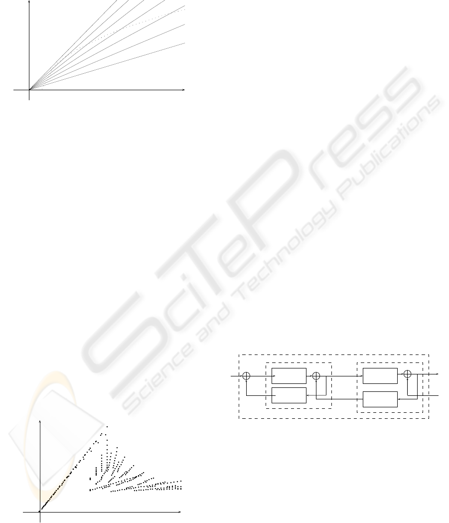
These values are respectively proportional to the ve-
hicles density K and the flow Q. We then obtain the
fundamental diagram of figure 5.This diagram gives
the relation between the flow and the vehicles den-
sity for the car traffic on a road. It has been observed
empirically and derived theoretically in the case of a
unique road or a regular system of roads (see for ex-
ample (Helbing, 2001)).
Q
K(v.m
−1
)
(v.s
−1
)
0
Figure 5: Fundamental diagram obtained for a simple road
section.
Let us mention that with this model if signal u
a
1
is such that lim
t→∞
u
a
1
(t) − β
1
(t) = +∞, then since
y
a
1
(t) = min
s≤t
(β
1
(t − s) + u
a
1
(s)) ≤ β
1
(t) we have
lim
t→∞
u
a
1
(t) − y
a
1
(t) ≥ lim
t→∞
u
a
1
(t) − β
1
(t) = +∞.
This means that if the arrival of vehicles on the
road exceeds its service capacity then the section will
asymptotically contain an infinity of vehicles. The
next example notably shows how to take into account
the intrinsic limited capacity of a section.
4.2 Succesion of Elementary Stretches
with Limited Capacities
We now consider two successive road sections as rep-
resented on figure 6. These roadway stretches mod-
eled by β
1
and β
2
are also supposed to be without any
facilities (no traffic light, . . .), but W
1
and W
2
have
been added to limit their capacities. More precisely,
the maximum amount of vehicles that section 1 can
contain is supposed to correspond to the integer W
1
.
We then have
∀t, u
a
1
(t) = min(u(t), y
a
1
(t) +W
1
),
in which u
a
1
(t) denotes the amount of vehicles likely
to enter section 1 up to time t. This leads to
∀t, u
a
1
(t) ≤ y
a
1
(t) +W
1
⇔ u
a
1
(t) − y
a
1
(t) ≤ W
1
which shows that the number of vehicles on the sec-
tion given by u
a
1
(t) − y
a
1
(t) is then well bounded by
W
1
.
Referring to equations (7) defining the generic model,
we deduce for i = 1, 2 that
Θ
i
= h
i
Σ
i
= e
Φ
i
= W
i
h
i
Γ
i
= W
i
.
h
1
u
a
1
W
1
y
a
1
y
b
1
u
b
1
h
2
u
a
2
W
2
y
a
2
y
b
2
u
b
2
section 1 section 2
S
u
Figure 6: Two successive road sections.
From results detailed in section 3.2, we can com-
pute the representation for the system resulting from
section 1 and 2 in cascade. Defining two mappings
β
1
and β
2
comparable (but different slopes) as that of
figure 3, we have simulated the system as in section
4.1. We then obtain two fundamental diagrams:
• diagram of figure 7 obtained for flows between u
and y
a
2
, with u(t) denoting the amount of vehicles
which have been candidates for entering section 1
up to time t;
ICINCO 2009 - 6th International Conference on Informatics in Control, Automation and Robotics
164

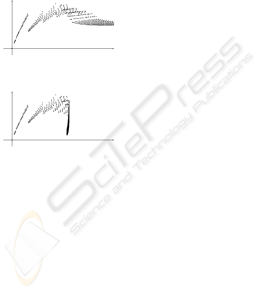
• diagram of figure 8 obtained for flows between u
a
1
and y
a
2
, with u
a
1
(t) denoting the amount of vehicles
having entered section 1 up to time t.
Q
(v.s
−1
)
K(v.m
−1
)
0
Figure 7: Fundamental diagram for two successive sections
with limited capacities (flows between u and y
a
2
).
Q
(v.s
−1
)
K(v.m
−1
)
0
Figure 8: Fundamental diagram for two successive sections
with limited capacities (flows between u
a
1
and y
a
2
).
5 DISCUSSION ON THE
PROPOSED (MIN,+) MODEL
For about fifty years, mathematical description of
traffic flow has been a lively subject of research and
debate for traffic engineers. This has resulted in a
broad scope of models describing different aspects of
traffic flow operations which can be classified accord-
ing to various criteria: level of detail, application area
and scale of application, deductive or inductive de-
scription of phenomena,...(see for example the survey
(Hoogendoorn and Bovy, 2001)). In this section, we
discuss the location of the proposed model in these
classifications.
Traffic flow can be described either by considering the
time-space behavior of individual drivers under the
influence of vehicles in their proximity (microscopic
models), the behaviour of drivers without explicitly
distinguishing their time-space behavior (mesoscopic
models), or from the viewpoint of the collective ve-
hicular flow (macroscopic models). According to the
level-of-detail, variables have different natures. In a
microscopicmodel variables describe individually be-
haviors and interactions of the systems entities (i.e.
vehicles and drivers). In macroscopic flow models,
the traffic stream is represented in an aggregate man-
ner using characteristics as flow-rate, density, and ve-
locity. In our model, we manipulate functions which
count every vehicle (from which we have derived ag-
gregated characteristics such as flow-rate and den-
sity), but their behavior is not necessarily described
individually through the approximation β of the im-
pulse response (unless the road section is sized such
that it contains only one vehicle). In that sense, our
model could be considered as an intermediate ap-
proach which, according to the size of the modeled
sections, fluctuates between microscopic and macro-
scopic approaches. Our description of observed phe-
nomena is also somewhat intermediate. In fact, the
choice of β and the limitation of capacity on sec-
tions come under a deductive approach of phenom-
ena which are known or which can be guessed. But
the mapping β should be the fitted thanks to an induc-
tive approach, that is using input/output data from real
systems.
Although it has only be used to simulate traffic flow
in the present paper, we expect that analytical results
can be derived from the proposed model. In fact,
for more than two decades a new system theory has
been developed for systems linear over idempotent
semi-rings (such as min-plus algebra): numerous re-
sults have been proposed for performance evaluation,
control,. . . (see (Cohen, 2006) for a recent survey).
In future works, some of these results should be ap-
plied/adapted to study vehicular traffic flow.
In this paper, we have considered elementary
stretches of roadways. On the one hand, we expect
that the chosen framework is sufficiently generic to
model a wide variety of more complex road sections
(with or without entry/exit lane, intersections, . . .).
On the other hand, the way to aggregate elementary
models is simple enough to consider that models for
large infrastructures can be obtained.
6 CONCLUSIONS
We have proposed a modeling method for traffic flow.
Each road section is modeled by its impulse response
in min-plus algebra. This model has been used to sim-
ulate and derive the fundamental diagram for elemen-
tary road stretches.
Future works will concern an identification method
to build an approximation β of the impulse response
from real road traffic data. We also plan to study more
A MIN-PLUS APPROACH FOR TRAFFIC FLOW MODELING
165

complex roadway stretches (for example phenomena
associated to a traffic light), and to adapt existing re-
sults from linear system theory over min-plus alge-
braic to derive analytical results on traffic flow.
REFERENCES
Baccelli, F., Cohen, G., Olsder, G. J., and Quadrat, J. P.
(1992). Synchronization and Linearity. Wiley.
Boudec, J. Y. L. and Thiran, P. (2001). Network Calculus:
A Theory of Deterministic Queuing Systems for the In-
ternet. Springer.
Cohen, G. (2006). A Tour of Systems with the Max-Plus
Flavor, volume 341 of Lecture Notes in Control and
Information Sciences, chapter Positive Systems, pages
19–24.
COINC, R.-G. (2009). Computational issues in network
calculus. http://perso.bretagne.ens-cachan.fr/˜ bouil-
lar/coinc/.
Cruz, R. L. (1991a). A calculus for network delay, part I:
Network elements in isolation. IEEE Transactions on
Information Theory, 37(1):114–131.
Cruz, R. L. (1991b). A calculus for network delay, part II:
Network analysis. IEEE Transactions on Information
Theory, 37(1):132–141.
Farhi, N., Goursat, M., and Quadrat, J. P. (2007). Road traf-
fic models using petri nets and minplus algebra. In
Proceedings of the Traffic and Granular Flow Confer-
ence, Orsay, Paris.
Gaubert, S. (1992). Th´eorie des syst`emes lin´eaires dans les
dioides. Th`ese. PhD thesis, Ecole des Mines de Paris.
Helbing, D. (1996). Gas-kinetic derivation of Navier-
Stokes-like traffic equations. Physical Review E,
53(3):2366–2381.
Helbing, D. (2001). Traffic and related self-driven
many-particle systems. Reviews of modern physics,
73:1067–1141.
Hoogendoorn, S. P. and Bovy, P. H. L. (2001). State-of-the-
art of Vehicular Traffic Flow Modelling. Journal of
Systems and Control Engineering, 215(4):283–303.
Lahaye, S. (2000). Contribution `a l’´etude des syst`emes
lin´eaires non stationnaires dans l’alg`ebre des dioides.
PhD thesis, Universit´e d’Angers.
Lolito, P., Mancinelli, E., and Quadrat, J. P. (2005). A Min-
plus Derivation of the Fundamental Car-Traffic Law.
IEEE Transactions on Automatic Control, 50(5):699–
705.
Menguy, E., Boimond, J. L., Hardouin, L., and Ferrier,
J. L. (2000). A First Step Towards Adaptative Con-
trol for Linear Systems in Max-Plus Algebra. Dis-
crete Event Dynamic Systems: Theory and Applica-
tions, 10(1):347–367.
Nagel, K. and Schreckenberg, M. (1992). A cellular
automaton model for freeway traffic. Journal de
Physique I France, 2(2):2221–2229.
ICINCO 2009 - 6th International Conference on Informatics in Control, Automation and Robotics
166