PARAMETER OPTIMIZATION IN TIME-FREQUENCY ε-FILTER

BASED ON CORRELATION COEFFICIENT

Tomomi Abe

Waseda university, 55N-4F-10A, 3-4-1 Okubo, Shinjuku-ku, Tokyo, 169-8555, Japan

Mitsuharu Matsumoto

The University of Electro-Communications, 1-5-1, Chofugaoka, Chofu-shi, Tokyo, 182-8585, Japan

Shuji Hashimoto

Waseda university, 55N-4F-10A, 3-4-1 Okubo, Shinjuku-ku, Tokyo, 169-8555, Japan

Keywords:

Noise reduction, Parameter optimization, ε-ﬁlter, Time-frequency domain.

Abstract:

Time-Frequency ε-ﬁlter (TF ε-ﬁlter) can reduce most kinds of noise from a single-channel noisy signal with

preserving the signal that varies drastically such as a speech signal. The ﬁlter design is simple and it can

effectively reduce noise. It can reduce not only small stationary noise but also large nonstationary noise.

However, it has some parameters and we need to set them appropriately based on empirical control. So far,

there are few studies to evaluate the appropriateness of the parameter setting of ε-ﬁlter in general. In this

paper, we employ correlation coefﬁcient of the ﬁlter output and the difference between the input and the ﬁlter

output as the evaluation function of the parameter setting. We also show the algorithm to set the optimal

parameter of TF ε-ﬁlter. We conducted the experiments to compare the value of the correlation coefﬁcient

and the mean square error when we change ε value. The experimental results show the applicability of our

criterion in parameter setting of ε-ﬁlter.

1 INTRODUCTION

Noise reduction plays an important role in speech

recognition and individual identiﬁcation. When

we consider the instruments like hearing-aids and

phones, noise reduction for a single-channel signal

is required. The spectral subtraction (SS) is a well-

known approach for reducing the noise signal of the

monaural-sound (Boll, 1979; Lim, 1978). It can re-

duce the noise effectively despite of the simple pro-

cedure. However, it can handle only the station-

ary noise. It also needs to estimate the noise in ad-

vance. Although noise reduction utilizing Kalman ﬁl-

ter has also been reported (Kalman, 1960; Fujimoto

and Ariki, 2002), the calculation cost is large. Some

authors have reported a model based approach for

noise reduction (Daniel et al., 2006). In this approach,

we can extract the objective sound by constructing the

sound model in advance. However, it is not applicable

to the signals with the unknown noise as well as SS.

There are some approaches utilizing comb ﬁlter (Lim

et al., 1978). In this approach, we ﬁrstly estimate the

pitch of the speech signal, and reduce the noise signal

utilizing comb ﬁlter. However, the estimation error

results in the degradation of the speech quality.

Some authors have reported a nonlinear ﬁlter

named ε-ﬁlter for noise reduction (Harashima et al.,

1982) with preserving the signal. We call it “TD ε-

ﬁlter” as it treats signal shape in time domain. TD

ε-ﬁlter is simple and has some desirable features for

noise reduction. It does not require the model not only

of the signal but also of the noise in advance. It is

easy to be designed and the calculation cost is small.

It can reduce not only the stationary noise but also the

nonstationary noise. However, it can reduce only the

small amplitude noise in principle. To solve the prob-

lems, the method labeled time-frequency ε-ﬁlter (TF

ε-ﬁlter) was proposed (Abe et al., 2007). TF ε-ﬁlter

is an improved ε-ﬁlter applied to the complex spec-

tra along the time axis in time-frequency domain. By

utilizing TF ε-ﬁlter, we can reduce not only small am-

plitude stationary noise but also large amplitude non-

stationary noise. However, TF ε-ﬁlter has some pa-

rameters and we need to set them adequately based

107

Abe T., Matsumoto M. and Hashimoto S. (2009).

PARAMETER OPTIMIZATION IN TIME-FREQUENCY -FILTER BASED ON CORRELATION COEFFICIENT.

In Proceedings of the International Conference on Signal Processing and Multimedia Applications, pages 107-111

DOI: 10.5220/0002182601070111

 SciTePress

on empirical control. Moreover, as we only have a

single-channel noisy signal, it is difﬁcult to evaluate

whether the parameter is optimal or not. We cannot

know the difference between the original signal and

the ﬁlter output from the observed signal. So far, there

are few studies on the appropriateness of the parame-

ter setting of ε-ﬁlter in general.

As a simple criterion, we assume that the signal

and noise are noncorrelated. And we employ the cor-

relation coefﬁcient of the ﬁlter output and the differ-

ence between the input signal and the ﬁlter output

to set ε adequately. We introduce a method to de-

termine the parameter utilizing the correlation coefﬁ-

cient. When we utilize the proposed method, we can

set the parameters adequately without the information

about the noise and the signal. In Sec.2, we explain

TF ε-ﬁlter to clarify the problem. In Sec.3, we de-

scribe the algorithm of the method to determine the

parameter adequately. In Sec.4, we show the exper-

imental results. Experimental results show that the

proposed method can estimate the optimal parameter

of the TF ε-ﬁlter. Conclusions are given in Sec.5.

2 TIME-FREQUENCY ε-FILTER

To clarify the problems of a TF ε-ﬁlter, we brieﬂy

explain the TF ε-ﬁlter algorithm. TF ε-ﬁlter utilizes

the distribution difference of the speech signal and

the noise in the frequency domain. The following as-

sumptions regarding the sound sources are used (Abe

et al., 2007):

• Assumption 1. Speech signal has greater vari-

ation in power than noise signal in the time-

frequency domain.

• Assumption 2. Noise signal is distributed more

uniformly and becomes less variation in the time-

frequency domain compared to in the time do-

main.

Figure 1 depicts the speech signal and the white noise

signal in the time and the time-frequency domains.

As shown in Figure 1, assumptions 1 and 2 are

fulﬁlled in the case of various noises like white noise

and natural noise such as the sound of a cooling fan.

In Figures 1(b) and (d), the power is normalized based

on the maximal power of the speech signal. When

we consider frequencybins correspondingto the pres-

ence of active speech signal, the power of the noise

with respect to the power of the signal is smaller than

the power of the noise with respect to the power of

the signal in the time domain. In TF ε-ﬁlter, we uti-

lize this feature to apply an ε-ﬁlter to high-level noise.

0 1 2

-0.4

-0.2

0.2

0.4

Time[s]

Amplitude

(a) Speech signal

(in time domain)

Time[s]

Power

0.5

x 10

Frequency[Hz]

(b)Speech signal (in

time-frequency domain)

0 1 2

-0.4

-0.2

0.2

0.4

Time[s]

Amplitude

(in time domain)

Power

Frequency[Hz]

Time[s]

0.5

x 10

(d) Noise signal

(in time-frequency domain)

Figure 1: A speech signal or noise signal in the time and

time-frequency domains.

Let us deﬁne x(k) as the input signal sampled at

time k. In TF ε-ﬁlter, we ﬁrstly transform the input

signal x(k) to the complex amplitude X(κ, ω) by short

term Fourier transformation (STFT). where κ and ω

represent the time frame in the time-frequency do-

main and the angular frequency, respectively. κ and ω

are discrete numbers. Next we execute a TF ε-ﬁlter,

which is an ε-ﬁlter applying to complex spectra along

the time axis in the time-frequency domain. In this

procedure, Y(κ, ω) is obtained as follows:

Y(κ, ω) =

∑

i=−Q

a(i)X

′

(κ+ i, ω), (1)

where the window size of ε-ﬁlter is 2Q+ 1,

′

(κ+ i, ω) (2)



X(κ, ω) (||X(κ, ω)| − |X(κ+i, ω)|| > ε)

X(κ +i, ω) (||X(κ, ω)| − |X(κ+i, ω)|| ≤ ε),

and ε is a constant.

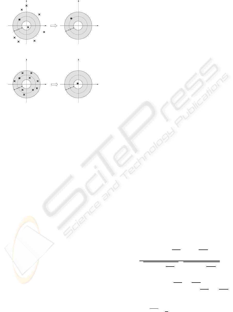
Figure 2 illustrates the differences in performance

when we apply a TF ε-ﬁlter to the speech signal and

the noise. The horizontal axis and the vertical axis

represent the real axis and the imaginary axis, respec-

tively. In the following explanations, we basically use

the word “signal” when we handle them as the sym-

bols while we use the word “complex spectra” when

we handle them as the values. We used the word “sig-

nal” as the mean of “all the signal points”. We also

used the word “complex spectra of the points” as the

“all the complex amplitudes of the points”. In Fig-

ure 2, ∗ and × represent the processed point and the

other signal points in the same window, respectively.

SIGMAP 2009 - International Conference on Signal Processing and Multimedia Applications

108

Im Im

(a) Speech signal

(b) Noise signal

Figure 2: Performance difference when a TF ε-ﬁlter is ap-

plied to the speech signal and noise.

Point A in Figure 2(a) and point B in Figure 2(b) rep-

resent the complex amplitude of the processed point.

′

and B

′

represent the complex amplitudes of the out-

puts when we apply the TF ε-ﬁlter to the points A and

B, respectively. Executing the TF ε-ﬁlter, we ﬁrstly

replace the complex amplitude of the signal outside

of the shadow area by that of A. We then summate

the complex spectra of all the points in the same win-

dow. Due to handling complex spectra, when we

have many signals that have similar powers but dif-

ferent phases, they are ﬁltered out by the TF ε-ﬁlter

and the complex amplitudes of the ﬁlter outputs be-

come small. Figure 2(a) represents the basic concept

in the case that the power varies frequently like in

a speech signal. When we consider a signal whose

power varies frequently, the difference between the

absolute value of A and that of the other signals is

large as shown in Figure 2(a). For this reason, many

signals in the same window as the point A are replaced

by A. As a result, when we handle the speech signal,

the complex amplitude of the processed point is al-

most preserved. Figure 2(b) represents the basic con-

cept in case that the power does not vary so much like

in a noise signal. When we consider a noise signal,

the difference between the absolute value of B and

that of the other signals is relatively small compared

with the speech signal. Hence, few signals in the same

window as point B are replaced by B. Based on these

aspects, we can reduce noise while preserving the sig-

nal by setting ε appropriately. Hence, the TF ε-ﬁlter

is effective even when the power of the noise with re-

spect to the power of the signal is large. Additionally,

under assumption 2, the TF ε-ﬁlter becomes more ef-

fective. When assumption 2 is satisﬁed, the variation

of the noise with respect to the variation of the sig-

nal in the frequency domain becomes smaller than the

case in the time domain. As a consequence, even if

the noise varies frequently in the time domain, the ε-

ﬁlter can be applied in the time-frequency domain.

Then, we transform Y(κ, ω) to y(k) by inverse

STFT.

In TF ε-ﬁlter, ε is an essential parameter to reduce

the noise appropriately. If ε is set to excessively large

values, the TF ε-ﬁlter becomes similar to linear ﬁlter

and smoothes not only the noise but also the signal.

On the other hand, if ε is set to an excessively small

value, it does nothing to reduce the noise anymore.

Due to these reasons, ε value should be set adequately.

3 PARAMETER OPTIMIZATION

UTILIZING CORRELATION

COEFFICIENT

As described in the previous section, when the TF ε-

ﬁlter is employed, we need to set ε value adequately

to reduce the noise. However, we cannot estimate op-

timal parameter because the noise and signal are not

known throughout all the procedures.

To solve the problem, we pay attention to the cor-

relation of the speech signal and the noise signal. We

make the following assumption concerning the sound

source and noise:

• Assumption 1. The speech signal is noncorre-

lated with the noise signal.

Let us deﬁne s(k) and n(k) as the objective signal

and the noise, respectively. Let R(s(k), n(k)) be the

correlation coefﬁcient of s(k) and n(k) described as

follows:

R(s(k), n(k))

∑

k=1

(s(k) −

s(k))(n(k) − n(k))

∑

k=1

(s(k) −

s(k))

∑

k=1

(n(k) −

n(k))

, (3)

where L is the data length.

s(k) and n(k) represent the

average of s(k) and n(k), respectively. s(k) and n(k)

are described as follows:

s(k) =

∑

k=1

s(k). (4)

PARAMETER OPTIMIZATION IN TIME-FREQUENCY W-FILTER BASED ON CORRELATION COEFFICIENT

109

n(k) =

∑

k=1

n(k). (5)

When L is large enough, it is expected that the as-

sumption 1 satisﬁes:

R(s(k), n(k)) = 0. (6)

As described above, s(k) and n(k) are unknown

throughout the ﬁltering procedures. Instead of s(k)

and n(k), we consider the correlation coefﬁcient of

the ﬁlter output and the difference between the input

signal and the ﬁlter output. Let us consider x(k) and

y(k) as the input signal and the output signal of TF ε-

ﬁlter, respectively. x(k) can be described as follows:

x(k) = s(k) + n(k). (7)

When the TF ε-ﬁlter can reduce the whole noise,

while it preserves the signal completely, the ﬁlter out-

put y(k) equals the signal s(k). The noise n(k) can be

described as follows:

n(k) = x(k) − s(k)

= x(k) − y(k). (8)

Although actual TF ε-ﬁlter does not reduce the

whole noise and also reduces the signal, if ε value

is set optimally, it is expected that the correlation co-

efﬁcient of y(k) and x(k) − y(k), R(y(k), x(k) − y(k))

has a smaller value than R(y(k), x(k) − y(k)) in other

ε. Hence, the optimal parameter ε

opt

can be obtained

opt

= argmin

R(y(k), x(k) − y(k)), (9)

where

R(y(k), x(k) − y(k)) (10)

∑

k=1

(y(k) −

y(k))(x(k) − y(k) − x(k) − y(k))

∑

k=1

(y(k) −

y(k))

∑

k=1

(x(k) − y(k) −

x(k) − y(k))

where

x(k) and x(k) − y(k) represent the aver-

age of x(k) and x(k) − y(k), respectively. x(k) and

x(k) − y(k) are described as follows:

x(k) =

∑

k=1

x(k). (11)

x(k) − y(k) =

∑

k=1

(x(k) − y(k)). (12)

We test its adequateness in the following section.

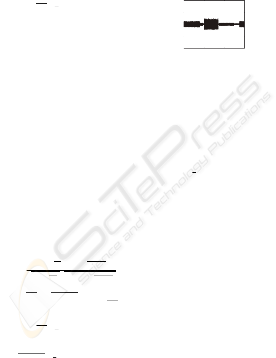
0 1 2

-0.4

-0.2

0.2

0.4

Time[s]

Amplitude

Figure 3: Waveform of the nonstationary noise.

4 EXPERIMENT

4.1 Experimental Condition

To clarify the adequateness of the proposed method,

we conducted the experiments utilizing a speech sig-

nal with a noise signal. In the experiments, we cal-

culate R(y(k), x(k) − y(k)) and the mean square error

(MSE) between the original signal s(k) and the ﬁlter

output y(k). MSE is deﬁned as follows:

MSE =

∑

k=1

(s(k) − y(k))

. (13)

As the sound source, we used “Japanese Newspa-

per Article Sentences” edited by the Acoustical Soci-

ety of Japan. We used the white noise with uniform

distribution as the stationary noise. As nonstation-

ary noise, we prepared white noise with the ampli-

tude that sometimes varied as shown in Figure 3. The

signal and the noise are mixed in the computer. The

sampling frequency and quantization bit rate are set at

44.1kHz and 16bits, respectively. We set the window

size of TF ε-ﬁlter at 61.

4.2 Relation between the MSE and the

Correlation Coefﬁcient

We prepared two noisy signals with stationary noise

and nonstationary noise whose SNR are 10.0[dB]. We

applied the ε-ﬁlter to the signals with changingε value

with range[0.1, 0.5].

Figures 4 and 5 show the experimental results

when we use the signal with stationary noise and non-

stationary noise as the input signal, respectively. As

shown in Figures 4 and 5, the ε value that has the

minimal value of correlation coefﬁcient corresponds

to the ε value that has the minimal value of MSE in

both cases. We could obtain similar results when we

utilized other signals.

SIGMAP 2009 - International Conference on Signal Processing and Multimedia Applications

110

0.05

0.1

0.15

0.2

0.25

0.3

0.35

0.1 0.3 0.5 0.7 0.9 1.1 1.3 1.5

Correlation coefficient

0.05

0.1

0.15

0.2

0.25

0.3

Mean square error[x10 ]

Correlation

coefficient

Mean square

error

-3

Figure 4: Experimental result when we used the signal with

stationary noise.

0.05

0.1

0.15

0.2

0.25

0.3

0.35

0.1 0.3 0.5 0.7 0.9 1.1 1.3 1.5

Correlation coefficient

0.05

0.1

0.15

0.2

0.25

0.3

0.35

Mean square error[x10 ]

Correlation

coefficient

Mean square

error

-3

Figure 5: Experimental result when we used the signal with

nonstationary noise.

5 CONCLUSIONS

In this paper, we employed correlation coefﬁcient of

the ﬁlter output and the difference between the input

and the ﬁlter output as the evaluation function of the

parameter setting of TF ε-ﬁlter. We also introduced

an algorithm to determine the parameter of TF ε-ﬁlter

automatically. The experimental results showed that

we can determine the parameter of TF ε-ﬁlter ade-

quately by utilizing our criterion. We can employ

ε value which has the minimal value of correlation

coefﬁcient between x(k) and x(k) − y(k) when TF ε-

ﬁlter is used. As the proposed method only assumes

the decorrelation of the signal and noise, it is expected

that the application range of the proposed method

is wide. By using our method, even when we only

have the single-channel noisy signal, we can evaluate

whether the ε value is adequate or not. The proposed

method does not require to estimate the noise in ad-

vance. For future works, we would like to evaluate the

robustness for changing the window size of the TF ε-

ﬁlter. We also would like to determine all parameters,

that is, not only the ε value but also the window size

adequately based on automatic control. Adaptive TF

ε-ﬁlter, which can change its parameter adaptively de-

pending on the input signal, will be developed in the

near future.

ACKNOWLEDGEMENTS

This research was supported by the research grant

of Support Center for Advanced Telecommunications

Technology Research (SCAT), by the research grant

of Foundation for the Fusion of Science and Tech-

nology, and by the Ministry of Education, Culture,

Sports, Science and Technology, Grant-in-Aid for

Young Scientists (B), 20700168, 2008. This research

was also supported by the CREST project ”Founda-

tion of technology supporting the creation of digi-

tal media contents” of JST, by the Grant-in-Aid for

the WABOT-HOUSE Project by Gifu Prefecture, and

the Global-COE Program,” Global Robot Academia”,

Waseda University.

REFERENCES

Abe, T., Matsumoto, M., and Hashimoto, S. (2007). Noise

reduction combining time-domain ε-ﬁlter and time-

frequency ε-ﬁlter. In J. of the Acoust. Soc. America.,

volume 122, pages 2697–2705.

Boll, S. F. (1979). Suppression of acoustic noise in speech

using spectral subtraction. In IEEE Trans. Acoust.

Speech Signal Process., volume ASSP-27, pages 113–

120.

Daniel, P., Ellis, W., and Weiss., R. (2006). Model-based

monaural source separation using a vector-quantized

phase-vocoder representation. In Proc. IEEE Int’l

Conf. on Acoustics, Speech, and Signal Process. 2006.

Fujimoto, M. and Ariki, Y. (2002). Speech recognition un-

der noisy environments using speech signal estimation

method based on kalman ﬁlter. In IEICE Trans. Infor-

mation and Systems, volume J85-D-II, pages 1–11.

Harashima, H., Odajima, K., Shishikui, Y., and Miyakawa,

H. (1982). ε-separating nonlinear digital ﬁlter and its

applications. In IEICE trans on Fundamentals., vol-

ume J65-A, pages 297–303.

Kalman, R. E. (1960). A new approach to linear ﬁltering

and prediction problems. In Trans. of the ASME, vol-

ume 82, pages 35–45.

Lim, J. S. (1978). Evaluation of a correlation subtraction

method for enhancing speech degraded by additive

white noise. In IEEE Trans. Acoust. Speech Signal

Process., volume ASSP-26, pages 471–472.

Lim, J. S., Oppenheim, A. V., and Braida, L. (1978). Eval-

uation of an adaptive comb ﬁltering method for en-

hancing speech degraded by white noise addition. In

IEEE Trans. on Acoust. Speech Signal Process., vol-

ume ASSP-26, pages 419–423.

PARAMETER OPTIMIZATION IN TIME-FREQUENCY W-FILTER BASED ON CORRELATION COEFFICIENT

111