
PASSIVITY-BASED DYNAMIC BIPEDAL WALKING WITH
TERRAIN ADAPTABILITY
Dynamics, Control and Robotic Applications
Qining Wang, Long Wang, Jinying Zhu, Yan Huang and Guangming Xie
Intelligent Control Laboratory, College of Engineering, Peking University, Beijing 100871, China
Keywords:
Passive dynamic walking, Bipedal robots, Terrain adaptability, Modeling.
Abstract:
This paper presents an approach for passivity-based bipedal robots to achieve stable walking on uneven terrain.
A powered two-dimensional seven-link walking model with flat feet and compliant ankles has been proposed to
analyze and simulate the walking dynamics. We further describe an optimization based control method, which
uses optimized hip actuation and ankle compliance as control parameters of bipedal walking. Satisfactory
results of simulations and real robot experiments show that the passivity-based walker can achieve stable
bipedal walking with larger ground disturbance by the proposed method in view of stability and efficiency.
1 INTRODUCTION
Stability guaranteed dynamic bipedal walking is one
of the keys but also one of the more challenging com-
ponents of humanoid robot design. Several actively
controlled bipedal robots are able to deal with such
dynamic stability when walk on irregular surface (Ya-
maguchi and Takanishi, 1997), step over obstacles
(Guan et al., 2006), climb stairs (Michel et al., 2007),
even if achieve bipedal running (Honda Motor, 2005).
However, to increase the autonomy of the robot, the
locomotion efficiency, which is far from that of hu-
man motion, has to be improved.
As one of the possible explanations for the ef-
ficiency of the human gait, passive dynamic walk-
ing (McGeer, 1990) showed that a mechanism with
two legs can be constructed so as to descend a gentle
slope with no actuation and no active control. Sev-
eral studies reported that these kinds of walking ma-
chines work with reasonable stability over a range of
slopes (e.g. (McGeer, 1990), (Collins et al. 2001))
and on level ground with kinds of actuation added
(e.g. (Collins et al. 2005), (Wisse et al., 2007)) show
a remarkable resemblance to the human gait. In spite
of having high energetic efficiency, passivity-based
walkers have limits to achieve adaptive locomotion on
rough terrain, which is one of the most important ad-
vantages of the legged robots. In addition, these walk-
ers are sensitive to the initial conditions of walking.
To overcome such disadvantages, several studies
proposed quasi-passive dynamic walking methods,
which implement simple control schemes and actua-
tors supplementarily to handle ground disturbances.
For example, (Schuitema et al., 2005) described a
reinforcement learning based controller and showed
that the walker with such controller can maximally
overcome −10mm ground disturbance. (Tedrake et
al., 2004) presented a robot with a minimal number
of degrees of freedom which is still capable of stable
dynamic walking even on level ground and even up
a small slope. (Wang et al., 2006) designed a learn-
ing controller for a two-dimensional biped model with
two rigid legs and curved feet to walk on uneven
surface that monotonically increases from 12mm to
40mm with a 2mm interval. In these studies, passivity-
based walkers are often modeled with point feet or
round feet. And the control parameter only includes
hip actuation. None of them analyzed the stability or
adaptability in quasi-passive dynamic walking with
flat feet and ankle joint compliance which is more
close to human motion. In fact, flat feet can offer
the advantage of distributing the energy loss per step
over two collisions, at the heel and at the toe (Kwan
and Hubbard, 2007), (Ruina et al., 2005). More-
over, experiments on human subjects and robot proto-
types revealed that the tendon of the muscle in ankle
joint is one mechanism that favors locomotor econ-
omy (Fukunaga et al., 2001), (Wang et al., 2007). It is
predictable that by controlling and optimizing the hip
actuation and ankle compliance, the passivity-based
bipedal walker may achieve adaptive bipedal locomo-
tion with larger disturbance on uneven terrain.
29
Wang Q., Wang L., Zhu J., Huang Y. and Xie G. (2009).
PASSIVITY-BASED DYNAMIC BIPEDALWALKING WITH TERRAIN ADAPTABILITY - Dynamics, Control and Robotic Applications.
In Proceedings of the 6th International Conference on Informatics in Control, Automation and Robotics - Robotics and Automation, pages 29-36
DOI: 10.5220/0002184200290036
Copyright
c
SciTePress
In this paper, we investigate how to control
passivity-based bipedal walkers to achieve stable
walking with terrain adaptability. A powered two-
dimensional seven-link walking model with flat feet
and ankle compliance has been proposed to analyze
and simulate the walking dynamics. We hypothesized
that the nervous system that controls human locomo-
tion may use optimized hip actuation and joint com-
pliance to achieve stable bipedal walking on irregular
terrain. Actually, hip actuation will cause the walker
to change locomotive patterns. Furthermore, we use
both simulations and real robot prototype to explore
the performance of the passivity-based walkers when
walk on uneven terrain by utilizing a biologically in-
spired optimization based controller, which is adap-
tive and capable of selecting proper hip actuation and
ankle compliance in view of walking stability and ef-
ficiency.
This paper is organized as follows. Section II de-
scribes the walking dynamics of the biped with flat
feet and ankle compliance. In Section III, we present
the optimization based walking control method. In
section IV, experimental results of stable locomotion
with terrain adaptability are shown. We conclude in
Section V.
2 PASSIVITY-BASED BIPEDAL
WALKER
Our model extended the Simplest Walking Model
(Garcia et al., 1998) with the addition of hip joint
actuation, upper body, flat feet and linear spring
based compliance on ankle joints, aiming for adap-
tive bipedal locomotion with optimization based con-
troller. The model consists of an upper body (point
mass added stick) that rotates around the hip joint, a
point mass representing the pelvis, two legs with knee
joints and ankle joints, and two mass added flat feet
(see Fig. 1).
The mass of each leg is simplified as point masses
added on the Center of Mass (CoM) of the shank
and the thigh respectively. Similar to (Wisse et al.,
2004), a kinematic coupling has been used in the pro-
posed model to keep the body midway between the
two legs. In addition, our model added compliance
in ankle joints. Specifically, the ankle joints are mod-
eled as passive joints that are constrained by linear
springs. The model is implemented in MATLAB, us-
ing the parameter values shown in Table 1, which are
derived from the mechanical prototype.
The passive walker travels forward on level
ground. The stance leg keeps contact with the ground
while the swing leg pivots about the constraint hip.
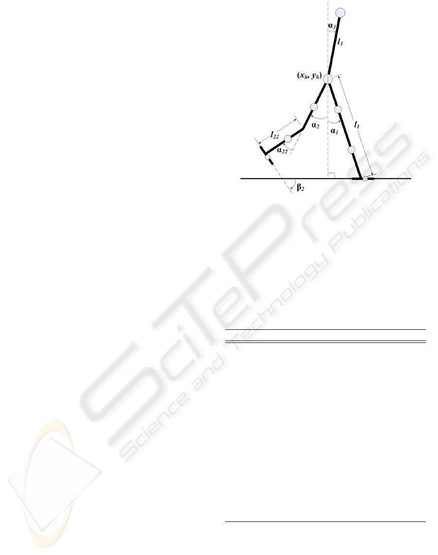
Figure 1: Two-dimensional seven-link passive dynamic
walking model. Mechanical energy consumption of level
ground walking is compensated by applying a hip torque.
The global coordinates of the hip joint is notated as (x
h
, y
h
).
α
1
and α
2
are the angles between each leg and the vertical
axis in sagittal plane respectively. The knee joints and an-
kle joints are all passive joints. To simulate human ankle
compliance, the ankle joints of the model are constrained
by linear springs.
Table 1: Default Parameter Values for the dynamic walking
model and the following simulations.
Parameter Description Value
m
1
, m
2
leg mass 1.12kg
m
3
upper body mass 0.81kg
m
4
hip mass 15.03kg
m
1t
, m
2t
thigh mass 0.56kg
m
1s
, m
2s
shank mass 0.56kg
m
f 1
, m
f 2
foot mass 2.05kg
l
1
, l
2
leg length 0.7m
l
11
, l
22
shank length 0.35m
l
f 1
, l
f 2
foot length 0.15m
l
b
upper body length 0.5m
l
w
body width 0.15m
c
b
CoM of upper body 0.2m
c
1
, c
2
CoM of leg 0.2m
c
11
, c
22
CoM of shank 0.2m
k ankle stiffness 8.65Nm/rad
P hip torque 0.38Nm
To compensate the mechanical energy consumption,
similar to (Kuo, 2002), we added a hip torque P be-
tween the swing leg and the stance leg. When the flat
foot strikes the ground, there are two impulses, ”heel-
strike” and ”foot-strike”, representative of the initial
impact of the heel and the following impact as the
ICINCO 2009 - 6th International Conference on Informatics in Control, Automation and Robotics
30

whole foot contacts the ground.
The walking model can be defined by the rectan-
gular coordinates x which can be described by the x-
coordinates and y-coordinates of the mass points and
the corresponding angles. The walker can also be de-
scribed by the generalized coordinates q. The springs
on the ankles constrain the foot vertical to the shank
when no heel-strike or foot-strike has occurred.
2.1 Constraint Equations
The constraint equations ξ
1
and ξ
2
used to detect heel
contact with ground are defined as follows:
ξ
1
=
x
h
+ l
1
sinα
1
− l
f 1
cosα
1
− x
f 1
y
h
− l
1
cosα
1
− l
f 1
sinα
1
ξ
2
=
x
h
+ l
2
sinα
2
− l
f 2
cosα
2
− x
f 2
y
h
− l
2
cosα
2
− l
f 2
sinα
2
(1)
where x
f 1
and x
f 1
are the global x-coordinates of the
latest strike. When the flat foot completely contacts
the ground, the constraint equations ξ
3
and ξ
4
used
to maintain foot contact with ground are defined as
follows:
ξ
3
=
x
h
+ l
1
sinα
1
− x
f 1
y
h
− l
1
cosα
1
ξ
4
=
x
h
+ l
2
sinα
2
− x
f 2
y
h
− l
2
cosα
2
(2)
If only the heel contacts the ground, the constraint
equations ξ
5
and ξ
6
during the period before foot-
strike are defined as follows:
ξ
5
= (x
h
+ l
1
sinα
1
− x
f 1
)
2
+ (y
h
− l
1
cosα
1
)
2
− l
2
f 1
ξ
6
= (x
h
+ l
2
sinα
2
− x
2
)
2
+ (y
h
− l
2
cosα
2
)
2
− l
2
f 2
(3)
Note that ξ
5
and ξ
6
are similar to constraining the an-
kle joint that connects shank and foot to move in a
circular orbit with heel as the center and distance be-
tween heel and ankle joint as the radius.
Similar to (Wisse et al., 2004), a reduced mass ma-
trix M
r
is introduced, which is defined as follows:
[M
r
] = [T ]
T
[M
g
][T ] (4)
where the Jacobian T =
∂x
∂q
. Here x is the global co-
ordinates of the six pointmasses (stance shank with
foot, swing shank with foot, hip, stance thigh, swing
thigh, body), while M
g
is the mass matrix in global
coordinates. Matrix Ξ
i
transfers the independent gen-
eralized coordinates q into the constraint equation ξ
i
,
where i = 1,2,. . . , 6
Ξ
i
=
dξ
i
dq
(5)
Consequently, matrix
˜
Ξ
i
is defined as follows:
˜
Ξ
i
=
∂(Ξ
i
˙q)
∂q
˙q (6)
2.2 Single Support Phase
Suppose that leg 1 (l
1
) is the stance leg, while leg 2
(l
2
) is the swing leg. In the beginning of the single
support phase, the knee joint is locked (keep the shank
and the thigh in a straight line). The Equation of Mo-
tion (EoM) is described as follows:
M
r
Ξ
T
3
Ξ
3
0
¨q
F
c
=
F
r
−
˜
Ξ
3
(7)
where F
r
is the external force, while F
c
is the foot con-
tact force. Here, the external force F
r
is used to com-
pensate the mechanical energy consumption of level
ground walking, which defined as follows:
{F
r
} = [T ]
T
({F} − [M
g
]{ ¨x})
where F is the external force in global coordinates,
including gravity, hip actuation, and torque in com-
pliant ankle joints. Then when the swing leg is swung
forward, the knee joint releases the shank.
2.3 Heel-strike Phase
In this phase, leg 1 (l
1
) is still the stance leg, while leg
2 (l
2
) is the swing leg. The heel contacts the ground
(heel-strike occurs). The EoM of the model changes
to:
M
r
Ξ
T
6
Ξ
6
0
˙q
+
F
c
=
M
r
˙q
−
−eΞ
6
˙q
−
(8)
After the heel-strike, the foot rotates around the ankle
joint. The EoM of the model is:
M
r
Ξ
T
3
Ξ
T
6
Ξ
3
0 0
Ξ
6
0 0
¨q
F
c1
F
c2
=
F
r
−
˜
Ξ
3
−
˜
Ξ
6
(9)
Note that the constraint equations guarantee that the
stance leg maintains foot contact with ground and the
swing leg maintains heel contact with ground. In ad-
dition, the spring constant k in the compliant ankle
joints should not be too big. Otherwise, the stance leg
will lose contact with ground. In this phase, since the
foot rotates around the ankle joint, the force generated
by the springs on the swing leg should be considered
as external force. Thus, in this event, the mass matrix
M would not include the point mass of the swing foot.
2.4 Toe-strike Impulse
The proposed walking model with flat feet introduces
a toe-strike impulse in addition to the heel-strike col-
lision. The EoM of the model is:
M
r
Ξ
T
4
Ξ
4
0
˙q
+
F
c
=
M
r
˙q
−
−eΞ
4
˙q
−
(10)
PASSIVITY-BASED DYNAMIC BIPEDALWALKING WITH TERRAIN ADAPTABILITY - Dynamics, Control and
Robotic Applications
31

0
0.2
0.4
0.6
0.8
1
−1.5
−1
−0.5
0
−2.5
−2
−1.5
−1
−0.5
0
0.5
α
1
(rad)
˙α
2
(rad /s )
˙α
1
(rad /s )
(a)
0 3 6 9 12 15 18 2121
0.25
0.3
0.35
0.4
0.45
0.5
0.55
0.6
time (sec)
walking velocity (m/s)
k=1.65 Nm/rad
k=8.65 Nm/rad
k=15 Nm/rad
k=25 Nm/rad
k=35 Nm/rad
stiff ankle
(b)
Figure 2: (a) Basin of attraction of the passive dynamic
walking model with flat feet and compliant ankles. The
blue layers of points represent horizontal slices of a three-
dimensional region of initial conditions that eventually re-
sult in the cyclic walking motion. The fixed point is indi-
cated with a red point, which is above one of the sample
slices. (b) Results of actively changing walking speed with
the same hip actuation and different ankle compliance (k
varies).
Note that in this phase, we consider that the ankle
joint of the swing leg is constrained to move in a cir-
cular orbit with toe as the center and distance between
toe and ankle joint as the radius. The force generated
by the spring on the swing leg should be considered
as external force, which can also be considered as the
constraint force of the circular orbit. After the toe-
strike, one step ends.
2.5 Effects of Hip Actuation and Ankle
Compliance
By application of the cell mapping method that has
been used in the several studies of passive dynamic
walking (e.g. (Wisse et al., 2004), (Wisse et al.,
2007)), we found that the model performs well in
the concept of global stability. The allowable er-
rors can be much larger than the results obtained in
(Wisse et al., 2004). This can be inspected by the
evaluation of the basin of attraction as shown in Fig.
2(a), which is the complete set of initial conditions
that eventually result in cyclic walking motion. One
can find that cyclic walking with initial conditions
in Table 1, emerges even if the initial step is nearly
fourfold as large, e.g. {α
1
(0) = 0.8,
˙
α
1
(0) = −2.3,
˙
α
2
(0) = −0.8}. It indicates that passive dynamic
walking with flat feet and ankle compliance may play
better on rough terrain with ground disturbance.
It has been examined that optimized hip actuation
can improve the stability of the passive walker (Kurz
and Stergiou, 2005). In addition, one can use the hip
actuation as the control parameter to achieve stable
walking on uneven terrain (Schuitema et al., 2005)-
(Ueno et al., 2006). In our model mentioned above,
ankle compliance k can also be used as a control pa-
rameter to affect the walking gait. As shown in Fig.
2(b), under the same change of hip actuation, different
ankle compliance reveals different responses in walk-
ing velocity transition. It indicates that more compli-
ance results in more visible sensitivity to the change
of hip torque. According to the analysis of basins of
attraction with different k (Wang et al., 2007), we find
that a relatively small k will lead to more stable points.
However, more compliance in ankle joints may result
in often falling backward during walking. Thus, op-
timized ankle compliance may result in a more stable
bipedal walking that allows larger disturbance.
3 OPTIMIZATION BASED
WALKING CONTROL
In order to optimize the hip actuation and ankle com-
pliance which affect walking gait as analyzed above,
Particle Swarm Optimization (PSO) has been chosen
with a focus lying on quickly finding suitable results,
in view of time-consuming and adaptivity of the gait.
In the realization of the PSO algorithm, a swarm of
N particles is constructed inside a D-dimensional real
valued solution space, where each position can be a
potential solution for the optimization problem. The
position of each particle is denoted as X
i
(0 < i < N).
Each particle has a velocity parameter V
i
(0 < i < N).
It specifies that the length and the direction of X
i
should be modified during iteration. A fitness value
attached to each location represents how well the lo-
cation suits the optimization problem. The fitness
value can be calculated by a fitness function of the
optimization.
In this study, we used adaptive PSO with changing
inertia weight. The update equation for velocity with
inertial weight is described as follows:
v
k+1
id
= wv
k
id
+ c
1
r
k
1d
(pbest
k
id
− x
k
id
) + c
2
r
k
2d
(gbest
k
d
− x
k
id
)
(11)
where w is the inertia weight. v
k
id
is one component
of V
i
(d donates the component number) at iteration
k. Similarly, x
k
id
is one component of X
i
at iteration
k. pbest
i
(0 < i < N) and gbest are the personal best
position and the global best position at each iteration
respectively. c
1
and c
2
are acceleration factors. r
1
and
r
2
are random numbers uniformly distributed between
0 and 1. Note that each component of the velocity has
new random numbers. In order to prevent particles
from flying outside the searching space, the ampli-
tude of the velocity is constrained inside a spectrum
[−v
max
d
, +v
max
d
].
ICINCO 2009 - 6th International Conference on Informatics in Control, Automation and Robotics
32

3.1 Fitness Function and Optimization
Process
For a specific passive walker, the mechanical param-
eters (length and mass distribution) are constant. To
control passive dynamic walking on uneven terrain,
we focus the control parameters on hip actuation P
and ankle compliance k. Then the two-dimensional
parameter space is (P, k). Here a set of parameters
stands for a particle of PSO. Since the walker will be
optimized with integration of stability and efficiency,
the fitness function is defined as follows:
σ = σ
s
+ γσ
e
(12)
where σ
s
and σ
e
are the fitness value to assess the sta-
bility and efficiency of each set of parameters respec-
tively. γ is the tuning factor to change the importance
of the two characteristics.
There are several methods to evaluate the stabil-
ity of the passive dynamic walking. In this study,
the stability will be quantified by the modulus of the
Jacobian matrix of the mapping function as defined
in (Wisse et al., 2004). Here, we notate the maxi-
mal eigenvalue as λ
m
, which represents the decreas-
ing speed of the deviation. The stability grades varies
for different sets of parameters even they all have a
stable fixed point. The smaller the λ
m
is, the faster the
deviation decreases and the more stable the walker is.
The similar conclusion can be obtained when all sets
of parameters only have an unstable fixed point. The
larger the λ
m
is, the more far from the stable state the
walker is. Then we define the fitness function of sta-
bility as the follows:
σ
s
=
1
λ
m
(13)
Similar to (Collins et al. 2005) and (Wisse et al.,
2004), the energetic efficiency of walking can be eval-
uated by the specific resistance as follows:
Θ =
E
MgL
(14)
where E is the cost of energy. In this study, the energy
cost is generated only by the hip torque. M is the total
mass of the model. g is the acceleration of gravity. L
is the length of distance the robot passed. Then the
fitness function can be defined as follows:
σ
e
=
1
Θ
=
Mgl
E
(15)
From (12), (13) and (15), we can obtain the whole
expression of the fitness function:
σ =
1
λ
m
+ γ
Mgl
E
(16)
Figure 3: The control scheme to overcome ground distur-
bance with optimized hip torque and ankle compliance.
Additionally, to evaluate the walking motion after
overcoming ground disturbance, we introduce an-
other expression of fitness function. We use further
walking distance d instead of the fitness efficiency σ
e
.
Then the fitness function can be rewritten as:
σ =
1
λ
m
+ γd (17)
3.2 Gait Controller with Optimized
Parameters
After analyzing the effects of hip actuation and an-
kle compliance in the stability and adaptability of the
passive dynamic walker, we select P and k as the gait
control input. The output of the optimization simula-
tor P
o
(t) and k
o
(t) are added to the current actual hip
actuation P
a
(t) and ankle compliance k
a
(t) (see Fig.
3).
This results in extra hip torque to move the swing
leg more forward and prevent tripping. The purpose
of the failure-detection block in Fig. 3 is to monitor
in simulations the foot contact and the knee locking
in order to detect whether walking failed. A failure
means that the robot fell either backward or forward
or that it started running (both feet leave contact with
ground). There is a active control counter module in
the diagram. It is used to count the times of applying
active control (increasing or decreasing P or k) during
one continuous walking. The output of this module
make the simulator change P or k. With the dynamic
model that adequately describing the real robot, an
adaptive optimizing control scheme can be done with-
out manually set to teach the robot and without the
robot damaging itself.
4 EXPERIMENTAL RESULTS
All the simulation experiments used the dynamic
model mentioned in Section II which was imple-
PASSIVITY-BASED DYNAMIC BIPEDALWALKING WITH TERRAIN ADAPTABILITY - Dynamics, Control and
Robotic Applications
33
1 2 3 4 5 6
0
3
6
9
12
15
generation
ground disturbance (mm)
adaptable disturbance
Figure 4: Maximum ground disturbance with optimized hip
torque and ankle compliance that keep unchanged during
stable walking.
mented in MATLAB, using the parameter values
shown in Table 1. The numerical integration of the
second order differential EoMs uses the Runge-Kutta
method, which is similar to the simulation methods
mentioned in (Wisse et al., 2004).
4.1 Parameter Optimization
Based on the adaptive PSO with proper inertial weight
mentioned above, we optimized the hip torque (hip
actuation) and ankle compliance to achieve adaptive
walking with maximal allowable ground disturbance
of the model with parameter values in Table 1. The
testing scenario is a floor with one step down. The
height of the step is gradually chosen from the range
from 1mm to 20mm. The initial particles which rep-
resent the parameter set of P and k are randomly se-
lected from the corresponding points in 2(a) that will
finally achieve stable walking. During the walking
simulation of the dynamic model, the ground distur-
bance gradually increase. The optimization process
evaluates the maximum ground disturbance of the dy-
namic model with certain P and k. During the walk-
ing, the selected P and k keep constant to overcome
gradually increased ground disturbance. The opti-
mization finally record the maximum ground distur-
bance in each generation. The fitness function is (16).
Fig. 12 shows the results. It is clear that by apply-
ing the adaptive PSO, the optimization process can
quickly find the optimal parameter set. It also in-
dicated that with optimized hip actuation and ankle
torque, the passive dynamic walker can achieve stable
walking with no active control even if there is −11mm
ground disturbance.
4.2 Walking on Uneven Terrain with
Control
Starting from the optimized P and k with no active
control during walking simulations, we add the con-
trol scheme shown in Fig. 3 to the walking motion.
(a)
−0.4 −0.2 0 0.2 0.4 0.6 0.8 1
−4
−3
−2
−1
0
1
2
3
4
angle of thigh (rad)
angular velocity of thigh (rad/s)
(b)
−1.2 −1 −0.8 −0.6 −0.4 −0.2 0 0.2 0.4 0.6
−10
−5
0
5
10
15
20
25
angular velocity of shank (rad/s)
angle of shank (rad)
(c)
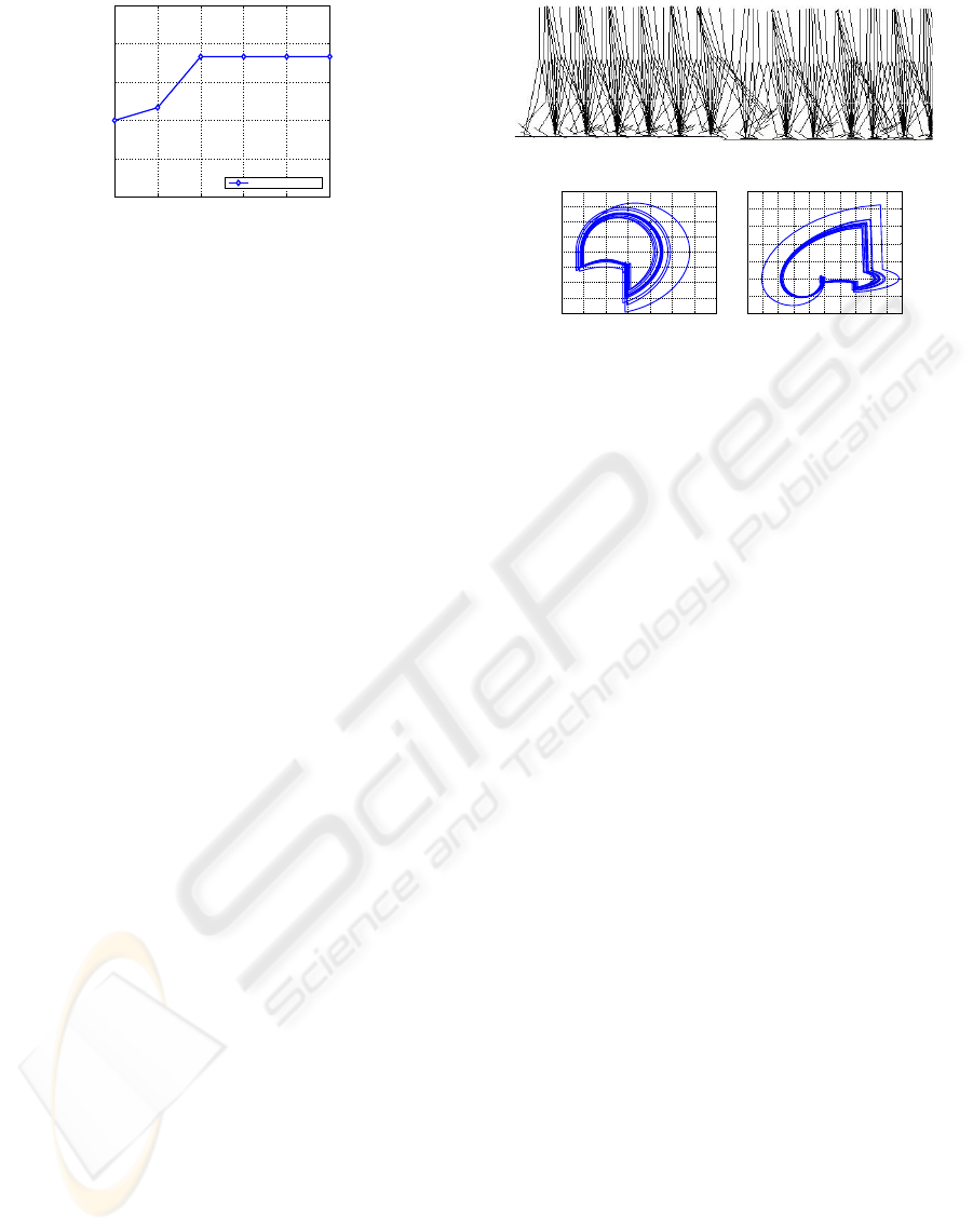
Figure 5: Adaptive locomotion with active control on un-
even terrain. This result is obtained every 10 frames during
a continuous walking. (a) is the stick diagram. (b) and (c)
are the angular trajectories of the thigh and shank respec-
tively.
A preset ground disturbance occurs at known time
during the level walking. The active control counter
determines the times of active control to change P
and k. In this simulation, the ground disturbance
varies from −15mm to −25mm. The fitness function
of the optimization is (17). The counter first makes
the optimization simulator to actively change P and
k once when ground disturbance occurs. There was
no optimized set of P and k that can overcome the
−25mm step. Then the counter makes the simulator
to actively change P and k twice when ground distur-
bance occurs. The walker successfully achieved sta-
ble walking with −25mm disturbance (see stick dia-
gram shown in Fig. 5(a)). Fig. 5(b) and (c) show the
trajectories of hip and knee during the adaptive walk-
ing.
Note that the cyclic walking was initially actuated
by a relatively small hip torque. After one time of ac-
tive control (varying P and k), the hip torque increased
to move the swing leg more forward and prevent trip-
ping. Since there was a second time of active con-
trol, the trajectories of the swing thigh and the swing
shank transited to bigger limit cycles. Such optimized
P and k finally stabilized the walking motion after a
step down occurred.
Fig. 6 shows the optimization process of the
hip actuation and ankle compliance during the walk-
ing with two times of active control. We set that if
the walker can walk stably for enough time after the
ground disturbance, the walking motion is adaptive
on the uneven ground. Specifically, the distance is
the product of walking speed times 25 seconds. Fig.
6(a) demonstrates the results of further distance after
ground disturbance each generation. After four gen-
ICINCO 2009 - 6th International Conference on Informatics in Control, Automation and Robotics
34

1 2 3 4 5 6 7 8 9
0
1
2
3
4
5
6
7
generation
further distance (m)
(a)
17.6
17.8
18
18.2
18.4
18.6
14.5
15
15.5
16
0
1
2
3
4
5
6
7
hip torque (Nm)ankle compliance (Nm/rad)
further distance (m)
(b)
Figure 6: Optimization of hip actuation and ankle compli-
ance. Both P and k vary during the continuous walking.
(a) is the results of further distance after ground disturbance
each generation. (b) is the results of selecting hip actuation
and ankle compliance during optimization.
erations, the walker can find optimized parameters to
overcome the step. Fig. 6(b) shows the process of
selecting P and k during the optimization. The ini-
tial hip torque is 5.5130Nm and ankle compliance is
12.2218Nm/rad. The two times of variance of P and
k are (18.0000Nm, 16.0000Nm/rad and (5.5000Nm,
15.4228Nm/rad) respectively.
Though there is no complex learning algorithm
in the control scheme, the walker can perform better
terrain adaptability comparing with other simulation
results (e.g. (Schuitema et al., 2005), (Wang et al.,
2006)).
4.3 Real Robot Experiments
To study natural and energy-efficient bipedal walking,
we designed and constructed a bipedal robot proto-
type, 1.2m in height and 20kg in weight. With the bi-
secting hip mechanism similar to (Wisse et al., 2007),
the prototype has five Degrees of Freedom (DOFs).
Two commercial motors are used in the hip joints to
perform hip actuation. Each leg consists of a thigh
and a shank interconnected through a passive knee
joint that has a locking mechanism. Springs are in-
stalled between the foot and the plate that is pushing
the leg up while it is rotated around the ankle. To pre-
vent foot-scuffing, we modified the foot with arc in
the front and the back-end. Specific mechanical pa-
rameters are shown in Table 1. In the experiment, by
using the proposed method, the robot tried to walk on
natural ground outdoor. The natural ground is not a
strict continuous level floor, where random irregular-
ity of the ground and slight slippery occurred. Fig. 7
shows the result.
The robot can achieve three-dimensional sta-
ble walking on natural ground with more than 10
steps. Comparing to the results of terrain adapt-
ability of other real robot experiments (e.g. two-
dimensional walkers (Wisse et al., 2005), (Ueno et al.,
2006)), the successful three-dimensional walking of
the robot prototype shows that the quasi-passive dy-
Figure 7: A sequence of photos captured during au-
tonomous walking of the robot prototype on natural ground.
namic walker with optimized hip actuation and ankle
compliance can perform stable walking with larger
ground disturbance.
5 CONCLUSIONS
In this paper, we have investigated how to control
passivity-based bipedal walkers to achieve stable lo-
comotion with terrain adaptability. Satisfactory re-
sults of simulations and real robot experiments in-
dicated that having the fixed mechanical parameters
during walking, the passivity-based walker can walk
on uneven terrain with larger ground disturbance by
optimized hip actuation and ankle compliance in view
of walking stability and efficiency. In the future, more
real robot experiments will be continued to overcome
more complex ground disturbance.
ACKNOWLEDGEMENTS
The authors would like to thank M. Wisse for shar-
ing the simulation files of the simplest walking model.
This work was supported by the National Natural Sci-
ence Foundation of China (No. 60774089), National
High Technology Research and Development Pro-
gram of China (863 Program) (No. 2006AA04Z258)
and 985 Project of Peking University.
REFERENCES
S. Collins, M. Wisse, A. Ruina, A three-dimensional
passive-dynamic walking robot with two legs and
knees, International Journal of Robotics Research,
vol. 20, pp. 607-615, 2001.
S. Collins, A. Ruina, R. Tedrake, M. Wisse, Efficient
bipedal robots based on passive-dynamic walkers, Sci-
ence, vol. 307, pp. 1082-1085, 2005.
PASSIVITY-BASED DYNAMIC BIPEDALWALKING WITH TERRAIN ADAPTABILITY - Dynamics, Control and
Robotic Applications
35

R. Eberhart, J. Kennedy, Particle swarm optimization, Proc.
of the IEEE Conf. on Neural Network, 1995, pp. 1942-
1948.
T. Fukunaga, K. Kubo, Y. Kawakami, S. Fukashiro, H.
Kanehisa, C. N. Maganaris, In vivo behaviour of hu-
man muscle tendon during walking, Proc. Biol. Sci.,
vol. 268, pp. 229-233, 2001.
M. Garcia, A. Chatterjee, A. Ruina, M. Coleman, The sim-
plest walking model: stability, complexity, and scal-
ing, ASME Journal Biomechanical Engineering, vol.
120: pp. 281–288, 1998.
Y. Guan, E. S. Neo, K. Yokoi, and K. Tanie, Stepping over
obstacles with humanoid robots, IEEE Transactions
on Robotics, 22(5), pp. 958-973, 2006.
Honda Motor Co., Ltd. New asimo - running at
6km/h, http://world.honda.com/HDTV/ASIMO/New-
ASIMO-run-6kmh/, 2005.
M. Kwan, M. Hubbard, Optimal foot shape for a passive
dynamic biped, Journal of Theoretical Biology, vol.
248, pp. 331-339, 2007.
A. D. Kuo, Energetics of actively powered locomotion
using the simplest walking model, ASME Journal
Biomechanical Engineering, vol. 124, pp. 113-120,
2002.
M. J. Kurz, N. Stergiou, An artificial neural network that
utilizes hip joint actuations to control bifurcations and
chaos in a passive dynamic bipedal walking model,
Biol. Cybern., vol. 93, pp. 213-221, 2005.
T. McGeer, Passive dynamic walking, International Journal
of Robotics Research, vol. 9, pp. 68-82, 1990.
P. Michel, J. Chestnutt, S. Kagami, K. Nishiwaki, J.
Kuffner, and T. Kanade, GPU-accelerated real-time
3D tracking for humanoid locomotion and stair climb-
ing, Proc. of the IEEE/RSJ Int. Conf. on Intelligent
Robots and Systems, 2007, pp. 463–469.
A. Ruina, J. E. A. Bertram, M. Srinivasan, A collisional
model of the energetic cost of support work quali-
tatively explains leg sequencing in walking and gal-
loping, pseudo-elastic leg behavior in running and the
walk-to-run transition, Journal of Theoretical Biology,
vol. 237, no. 2, pp. 170-192, 2005.
E. Schuitema, D. Hobbelen, P. Jonker, M. Wisse, J. Karssen,
Using a controller based on reinforcement learning for
a passive dynamic walking robot, Proc. of the IEEE-
RAS Int. Conf. on Humanoid Robots, 2005, pp. 232-
237.
R. Smith, U. Rattanaprasert, and N. O’Dwyer, Coordination
of the ankle joint complex during walking, Huamn
Movement Science, vol. 20, pp. 447-460, 2001.
R. Tedrake, T. W. Zhang, M. F. Fong, H. S. Seung, Actu-
ating a Simple 3D Passive Dynamic Walker. In Proc.
IEEE Int. Conf. Robotics and Automation, 2004, pp.
4656-4661.
T. Ueno, Y. Nakamura, T. Takuma, K. Hosoda, T. Shibata
and S. Ishii, Fast and stable learning of quasi-passive
dynamic walking by an unstable biped robot based on
off-policy natural actor-critic, Proc. of the IEEE/RSJ
International Conference on Intelligent Robots and
Systems, 2006, pp. 5226-5231.
S. Wang, J. Braaksma, R. Babu ˇska, D. Hobbelen, Re-
inforcement learning control for biped robot walk-
ing on uneven surfaces, Proc. of the 2006 Interna-
tional Joint Conference on Neural Networks, 2006,
pp. 4173-4178.
Q. Wang, J. Zhu, L. Wang, Passivity-based three-
dimensional bipedal robot with compliant legs, Proc.
of the SICE Annual Conference, 2008.
M. Wisse, A. L. Schwab, F. C. T. Van der Helm, Passive
dynamic walking model with upper body, Robotica,
vol. 22, pp. 681-688, 2004.
M. Wisse, A. L. Schwab, R. Q. van der Linde, F. C. T.
van der Helm, How to keep from falling forward: el-
ementary swing leg action for passive dynamic walk-
ers, IEEE Transactions on Robotics, vol. 21, no. 3, pp.
393-401, 2005.
M. Wisse, G. Feliksdal, J. van Frankenhuyzen, B. Moyer,
Passive-based walking robot - Denise, a simple, effi-
cient, and lightweight biped, IEEE Robotics and Au-
tomation Magazine, vol. 14, no. 2, pp. 52-62, 2007.
J. Yamaguchi and A. Takanishi, Development of a leg part
of a humanoid robot - development of a biped walk-
ing robot adapting to the humans’ normal living floor,
Autonomous Robots 4(4), pp. 369-385, 1997.
ICINCO 2009 - 6th International Conference on Informatics in Control, Automation and Robotics
36
