
MIMO INSTANTANEOUS BLIND IDENTIFICATION BASED ON
STEEPEST DESCENT METHOD
Shen Xizhong, Hu Dachao
Mechanical & Electrical department, Shanghai Institute of Technology, Shanghai, China
Meng Guang
State Key Laboratory for Mechanical System and Vibration, Shanghai Jiao Tong University, Shanghai, China
Keywords: Instantaneous blind identification, Homogeneous system, Second order temporal statistics, Steepest descent
method, Nonlinear.
Abstract: This paper presents a new MIMO instantaneous blind identification algorithm based on second order
temporal property and steepest descent method. Second order temporal structure is reformulated in a
particular way such that each column of the unknown mixing matrix satisfies a system of nonlinear
multivariate homogeneous polynomial equations. The nonlinear system is solved by steepest descent
method. We construct a general goal of the system and convert the nonlinear problem into an optimal
problem. Our algorithm allows estimating the mixing matrix for scenarios with 4 sources and 3 sensors, etc.
Finally, simulations show its effectiveness with more accurate solutions than the algorithm with homotopy
method.
1 INTRODUCTION
Multiple-input multiple-output (MIMO)
instantaneous blind identification (MIBI) is one of
the attractive blind signal processing (BSP)
problems, where a number of source signals are
mixed by an unknown MIMO instantaneous mixing
system and only the mixed signals are available, i.e.,
both the mixing system and the original source
signals are unknown. The goal of MIBI is to recover
the instantaneous MIMO mixing system from the
observed mixtures of the source signals. In this
paper, we focus on developing a new algorithm to
solve the MIBI problem by using second-order
temporal structure and steepest descent method.
The greater majority of the available algorithms
is based on generalized eigenvalue decomposition or
joint approximate diagonalization of two or more
sensor correlation matrices for different lags and/or
times arranged in the conventional manner
This work has been supported by NSFC with NO.
10732060, Shanghai Leading Academic Discipline Project
with No. J51501, and also Shanghai Education with No.
ZX2006-01.
(Cichocki A et al. 2002) (Hua and Tugnait
2000)(Lindgren and Veen 1996). An MIBI based on
second order temporal structure (SOTS) (Laar et al.
2008) has been proposed, which arrange the
available sensor correlation values in a particular
fashion that allows a different and natural
formulation of the problem, as well as the estimation
of the more columns than sensors.
In this paper, we further develop the algorithm
proposed in Laar et al. 2008 to obtain more accurate
and robust solution with a new contrast function.
2 MIBI MODEL
Let us use the usual model (Laar et al. 2008)
(Cichocki and Amari 2002) (Yingbo Hua and
Tugnait J K 2000) (U Lindgren and van der Veen
1996) in MIBI problem as follows
(
)
(
)()
ttt=+xAsν (1)
where
[
]
1
,,
nm
m
×
=∈Aa a"\ is an unknown
mixing matrix with its
n -dimensional array
118
Xizhong S., Dachao H. and Guang M. (2009).
MIMO INSTANTANEOUS BLIND IDENTIFICATION BASED ON STEEPEST DESCENT METHOD.
In Proceedings of the International Conference on Signal Processing and Multimedia Applications, pages 118-121
DOI: 10.5220/0002185701180121
Copyright
c
SciTePress

response vectors
()
T
1jj nj
aa=a " , 1, 2, ,jm= " ,
() () () ()
T
12
,,,
m
tstst st=
⎡⎤
⎣⎦
s "
is the vector of
source signals,
() () ()
T
1
,,
n
tt t
νν
=
⎡
⎤
⎣
⎦
ν " is the
vector of noises, and
() () () ()
T
12
,,,
n
txtxt xt=
⎡⎤
⎣⎦
x " is the vector of
observations.
Without knowing the source signals and the
mixing matrix, the MIBI problem is to identify the
mixing matrix from the observations by estimating
A as
ˆ
A
.
The mixing matrix is identifiable in the sense of
two indeterminacies, which are unknown
permutation of indices of each column of the matrix
and its unknown magnitude (Laar et al. 2008)
(Cichocki and Amari 2002) (Yingbo Hua and
Tugnait J K 2000) (U Lindgren and van der Veen
1996). Assume that each column of
A
satisfy the
normalization conditions, i.e., on the unit sphere,
()
2
1
10; 1,2, ,
n
jj ij
i
Sajm
=
=−==
∑
a " . (2)
To solve the MIBI problem, we define the
following concepts Def 1~2 for the derivation of the
algorithm, and then make the following assumptions
AS 1~4 (Laar et al. 2008).
Def 1 Autocorrelation function
(
)
,
,
sii
rt
τ
of
()
,
i
st i∀∈` at time instant t and lag
τ
is defined
as
() ()( )
,
,E ,,
sii i i
rt stst t
τττ
−
∀∈
⎡⎤
⎣⎦
]
. (3)
Def 2 Cross-correlation function
(
)
,
,
sij
rt
τ
of
() ()
,,,
ij
st s t ij∀∈` at time instant t and lag
τ
is
defined as
() ()( )
,
,E ,,
sij i j
rt stst t
τττ
⎡⎤
−
∀∈
⎣⎦
]. (4)
AS 1 the source signals have zero cross-correlation
on the noise-free region of support (ROS)
Ω :
()
12
,12
,0,1
sjj
rt jjm
τ
=∀≤ ≠ ≤ . (5)
AS 2 the source autocorrelation functions are
linearly independent on the noise-free ROS
Ω
()
,
1
, 0 0, 1, 2, ,
m
jsjj j
j
rt j m
ξτ ξ
=
=⇒ = ∀=
∑
" (6)
AS 3 the noise signals have zero auto- and cross-
correlation functions on the noise-free ROS
Ω
:
()
12
,12
,0,1,
njj
rt jjm
τ
=∀≤ ≤. (7)
AS 4 the cross-correlation functions between the
source and noise signals are zero on the noise-free
ROS
Ω :
(
)
(
)
,,
,,0,
1,1
sij s ji
rt rt
in jm
νν
ττ
=
=
∀
≤≤ ≤ ≤
. (8)
The procedure of our proposed algorithm
includes two steps, that is, step 1 is that the problem
of MIBI is formulated as the problem of solving a
system of homogeneous polynomial equations; and
step 2 is that steepest descent method is applied to
solve the system of polynomial equations. We detail
these steps respectively in sections 3 and 4.
3 HOMOGENEOUS
POLYNOMIAL EQUATIONS
In this section, we will review the algebraic structure
of MIBI problem derived under the above
assumptions, and some details can be referred to
Laar et al 2008. The correlation values of the
observations are stacked as
(
)()
,11
,,
xx xNN
tt
ττ
◊
⎡
⎤
⎣
⎦
Rr r"
, (9)
where
(
)
(
)( )
,E
xNN N N N
ttt
ττ
=⊗−
⎡
⎤
⎣
⎦
rxx
, and
⊗
denotes Kronecker product. The homogeneous
polynomial equations of degree two are expressed as
◊
=
ΦA0. (10)
Here,
◊
A is the second-order Khatri-Rao
product of
A , which is defined as
[
]
11 mm◊
⊗⊗Aaa aa" , and
(
)
12
12
,
1, , ; , 1, ,
qii
qQii n
ϕ
==
=Φ
""
is a matrix with
2
Qn
×
dimensions where
()
,
1
1
2
Qnn rank
◊
⎡⎤
=+−
⎣⎦
x
R , of
which its rows form a basis for the nonzero left null
space
(
)
,x
◊
Ν R
. Therefore, there are
Q
equations
about each column of
A
in (10).
Φ can be calculated by SVD of
,
x
◊
R , and
split into signal and noise subspace parts as
TT
,xsss
ν
νν
◊
=+RUΣ VUΣ V . The left null space of
,
x
◊
R is
T
ν
=Φ U .
By eq.(10), the maximum number
max
M of
columns that can be identified with
n sensors
equals
()()
max
1
11
2
Mnnn
=
+− −. (11)
MIMO INSTANTANEOUS BLIND IDENTIFICATION BASED ON STEEPEST DESCENT METHOD
119

4 STEEPEST DESCENT METHOD
In this section, we summarize the main ideas behind
the so-called steepest descent method (Richard and
Faires 2001) that provides a deterministic means for
solving a system of nonlinear equations, and then we
employ the steepest descent method to solve the
equations in (10) to form our algorithm.
We expand the expression in (10) as
()
12 1 2
1212
;
;1,,
0;
1, , ; 1, ,
qj qiiijij
iiii n
faa
qQjm
ϕ
≤=
==
=∀=
∑
a
"
""
., (12)
and then define our optimal goal function when
combining the constraint in (2) as
() () ()
222
1
,
1, ,
Q
jqjjj
q
gf S
jm
γ
=
+
∀=
∑
aaa
"
. (13)
Here,
γ
is added as a homogeneous factor,
which is applied to make the different square items
in (13) well-proportioned, and in our algorithm we
set
0.1
γ
= . Notice that we don’t think it as a
penalty term for imposing the constraint for it just
adjust the constraint in (2) and (12) to have the same
level of function values. To satisfy the constraint (2)
we normalize
j
a in each iterative step to unit vector.
The direction of greatest decrease in the value
of
()
j
g a at
(
)
k
j
a with
k
-th iteration is the
direction given by its minus gradient
(
)
j
g−∇ a of
()
j
g a . The gradient is expressed as
() ()
()
T
2
jj
g∇=aJaFx. (14)
Here,
() () () ()
()
T
1
,, ,
Q
ffS
γ
=Fx x x x" , and
()
j
Ja is its Jacobian matrix. The objective is to
reduce
()
j
g a to its minimal value of zero, and an
appropriate choice for
()
j
g a is
( ) () ()
()
1kk k
jj j
g
α
+
=−∇aa a, (15)
where
()
()
1
0
arg min
k
j
g
α
α
+
= a is the critical point.
We can apply any single-variable function optimal
method to find the minimum value of
()
(
)
1k
j
g
+
a
by an appropriate choice for the value
α
. In our
algorithm, we use Newton’s forward divided-
difference interpolating polynomial, detailed in
Richard and Faires 2001.
We employ the initial solutions as equal
distributed vectors in the super space of
j
a . To
guarantee that all the local minimums of the
proposed algorithm are obtained, we can use 8 or
more initial solutions equal distributed in the super
space, and then find the correct solutions by
clustering method. For simplicity, we decide the
four correct solutions by their minimum distances
between each other.
5 SIMULATIONS
We adopt three mixtures of four speech signals the
same example as in Laar et al. 2008. For
convenience, we name our algorithm as MIBI
Steepest Descent and the algorithm in Laar et al.
2008 as MIBI Homotopy.
The speech signals are sampled as 8kHz,
consist of 10,000 samples with 1,250ms length, and
are normalized to unit variance
1
s
σ
= . The signal
sequences are partitioned into five disjoint blocks
consisting of 2000 samples, and for each block, the
one-dimensional sensor correlation functions are
computed for lags 1, 2, 3, 4 and 5. Hence, in total
for each sensor correlation functions 25 values are
estimated and employed, i.e., the employed noise-
free ROS in the domain of block-lag pairs is given
by
(
)
(
)
(
)()
{
}
1, 1 , , 1, 5 , 2,1 , , 5, 5Ω= "",
where the first index in each pair represents the
block index and the second the lag index. The
sensor signals are obtained from (1) with
34
×
mixing matrix,
0.6749 0.4082 0.8083 0.1690
0.5808 0.8165 0.1155 0.5071
0.4552 0.4082 0.5774 0.8452
−
⎡
⎤
⎢
⎥
=− −
⎢
⎥
⎢
⎥
−−
⎣
⎦
A
.
The noise signals are mutually statistically
independent white Gaussian noise sequences with
variances
2
1
ν
σ
=
. The signal-to-noise ratio (SNR)
is -1.23dB, which is quite bad. We set the maximum
iterative number is 30, and stop the iteration if the
correction of the estimated is smaller than a certain
tolerance 10
-3
.
Let
i
θ
be the included angle between the
j
-th
column of
A and its estimate. The estimated
mixing matrix is
SIGMAP 2009 - International Conference on Signal Processing and Multimedia Applications
120
10 20 30 40 50
0
20
40
60
80
Comparision of MIBI Steepest Descent with MIBI Homotopy
Included Angle/
°
10 20 30 40 50
0
20
40
60
80
10 20 30 40 50
0
20
40
60
80
Compared numbers
Included Angle/
°
10 20 30 40 50
0
20
40
60
80
Compared numbers
(TL)
(TR)
(BL)
(BR)
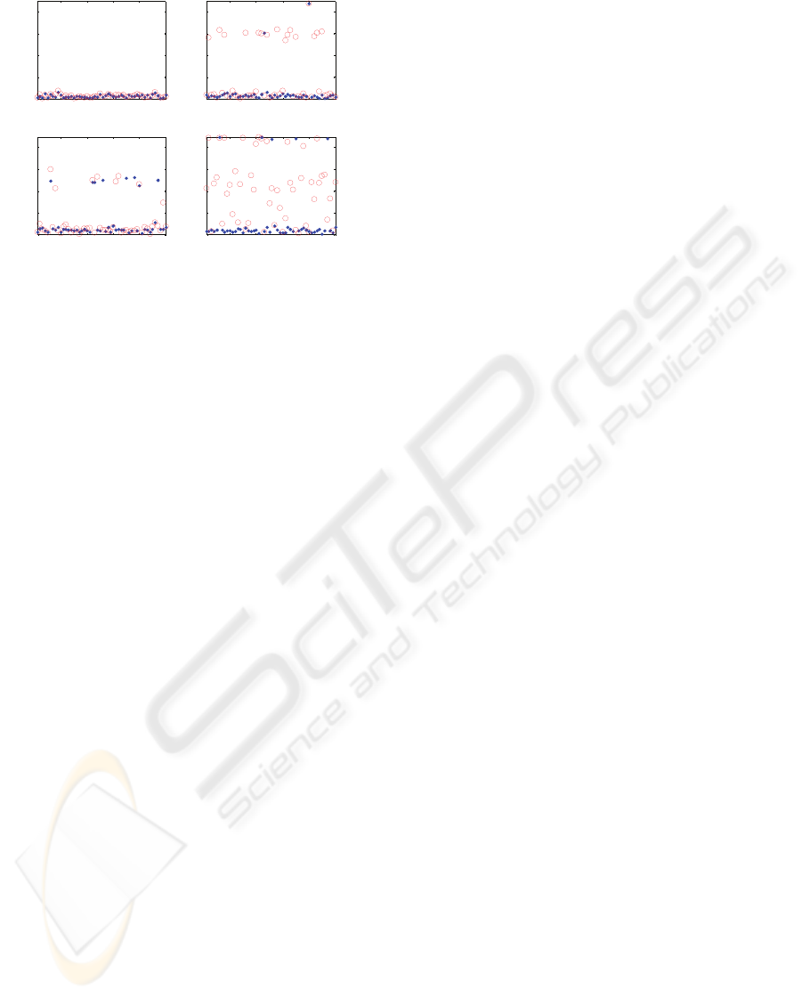
Figure 1: Comparisons of MIBI Steepest Descent with
MIBI Homotopy.
0.6542 0.4007 0.8239 0.1235
ˆ
0.5984 0.8152 0.0884 0.5343
0.4625 0.4183 0.5597 0.8362
−
⎡⎤
⎢⎥
=− −
⎢⎥
⎢⎥
−−
⎣⎦
A
,
and the included angles are 1.6120, 0.7214, 2.0583
and 3.0781. We see that the estimated columns
approximately equal the ideal ones.
Figure 1 shows the Comparisons of MIBI
Steepest Descent with MIBI Homotopy. TL, TR,
BL and BR in Figure 1 are respectively the
estimated included angles along different running
times between the first, second, third and fourth
columns and their estimates. Blue dot indicates the
result of MIBI_SD algorithm; and Red circle
indicates the results of MIBI_Homotopy algorithm.
We see that in TL and BL figure, the included angles
are almost the same with each other, but in TR and
BR figure, the estimates by MIBI Steepest Descent
are better than the ones by MIBI Homotopy.
Therefore, we conclude that the algorithm with
steepest descent has better performance than MIBI
Homotopy.
6 CONCLUSIONS
In this paper, we further develop the algorithm
proposed in Laar et al. 2008 to obtain more accurate
and robust solution with a new contrast function in
(13). SOTS is considered only on a noise-free
region of support. We project the MIBI problem in
(1) on the system of homogeneous polynomial
equations in (10) of degree two. Steepest descent
method is used for estimating the columns of the
mixing matrix, which is quite different from the
algorithm in Laar et al. 2008 which applied
homotopy method. This MIBI method presented in
this paper allows estimating the mixing matrix for
several underdetermined mixing scenarios with 4
sources and 3 sensors. Simulations show its
effectiveness with more accurate solutions.
REFERENCES
Cichocki A; Amari S I. Adaptive Blind Signal and Image
Processing: Learning Algorithms and Applications.
New York: Wiley, 2002.
van de Laar J; Moonen M; Sommen P C W. MIMO
Instantaneous Blind Identification Based on Second-
Order Temporal Structure. IEEE Transactions on
Signal Processing. Volume 56, Issue 9, Sept. 2008,
Page(s):4354 – 4364
Yingbo Hua; Tugnait, JK. Blind identifiability of FIR-
MIMO systems with colored input using second order
statistics. IEEE Signal Processing Letters, Volume: 7
Issue: 12, Dec 2000. Page(s): 348 -350.
U. Lindgren and A.-J. van der Veen, Source separation
based on second order statistics—An algebraic
approach. in Proc. IEEE SP Workshop Statistical
Signal Array Processing, Corfu, Greece, Jun. 1996, pp.
324–327.
Richard L. Burden; J. Douglas Faires. Numerical
Analysis. Thomson Learning. Inc. 2001, pp: 628-635.
MIMO INSTANTANEOUS BLIND IDENTIFICATION BASED ON STEEPEST DESCENT METHOD
121
