MODEL-ORDER REDUCTION OF SINGULARLY PERTURBED
SYSTEMS BASED ON ARTIFICIAL NEURAL ESTIMATION
AND LMI-BASED TRANSFORMATION
Othman M-K. Alsmadi, Za'er S. Abo-Hammour
Department of Electrical Engineering, University of Jordan, Amman, Jordan
Department of Mechatronics Engineering, University of Jordan, Amman, Jordan
Mohammad S. Saraireh
Department of Computer Engineering, Mutah University, Karak, Jordan
Keywords: Model order reduction, System transformation, Artificial neural networks, Linear matrix inequality (LMI),
Singular perturbation.
Abstract: A new method for model order reduction with eigenvalue preservation is presented in this paper. The new
technique is formulated based on the system state matrix transformation which preserves the system
eigenvalues and is accomplished using an artificial neural network training. A linear matrix inequality
(LMI) numerical algorithm technique is used to obtain the complete system transformation. Model order
reduction is then obtained utilizing the singular perturbation method. Simulation results show that the LMI-
based transformed reduced model order is superior to other reduction methods.
1 INTRODUCTION
The objective of any control system is to obtain a
desired response. In order to achieve this objective, a
dynamical model is usually developed based on a set
of differential equations (Franklin, 1994). The
obtained mathematical model may have a certain
parameter, called perturbation, that has a little effect
on the system performance (Kokotovic, 1986)
(Zhou, 2009). Neglecting this parameter results in
simplifying the order of the designed controller
based on reducing the system model order. A
reduced model order can be obtained by neglecting
the fast dynamics (i.e., non-dominant eigenvalues)
of the system and focusing on the slow dynamics
(i.e., dominant eigenvalues). This method is referred
to as singular perturbation. Simplification and
reduction of a system model leads to controller cost
minimization (Garsia, 1998). An example is the ICs,
where increasing package density forces developers
to include side effects. Knowing that these devices
are often modeled by large RLC circuits, this would
be too demanding computationally and practically
due to the detailed modeling of the original system
(
Benner, 2007). In control system, due to the fact that
feedback controllers do not usually consider all the
dynamics of the system, model reduction becomes a
very important issue (
Bui-Thanh, 2005).
For a reduced model order that will best mimic
the performance of its original system, system
transformation is performed. In the process of
system transformation, some system parameters are
required to be identified. This objective maybe
achieved by the use of artificial neural networks
(ANN) (Alsmadi, 2007), which are considered as the
new generation of information processing networks
(
Hinton, 2006). Artificial neural systems maybe
defined as physical cellular systems which have the
capability of acquiring, storing and utilizing
experiential knowledge. They can be represented as
mathematical or computational models based on
biological neural networks. An artificial neural
network consists of an interconnected group of
artificial neurons and processes information. They
perform summing operations and nonlinear function
computations. Neurons are usually organized in
layers and forward connections where computations
are performed in a parallel fashion at all nodes and
173
M-K. Alsmadi O., S. Abo-Hammour Z. and S. Saraireh M. (2009).
MODEL-ORDER REDUCTION OF SINGULARLY PERTURBED SYSTEMS BASED ON ARTIFICIAL NEURAL ESTIMATION AND LMI-BASED
TRANSFORMATION .
In Proceedings of the 6th International Conference on Informatics in Control, Automation and Robotics - Intelligent Control Systems and Optimization,
pages 173-180
DOI: 10.5220/0002187801730180
Copyright
c
 SciTePress

connections. Each connection is expressed by a
numerical value called a weight. The learning
process of a neuron corresponds to a way of
changing its weights. An artificial neural network
can be used to model complex relationships between
inputs and outputs of different systems (Haykin,
1994) (Zurada, 1992) (Williams, 1989).
In obtaining the overall transformed model,
which leads to control design advantages, part of the
transformation requires some optimized solution.
This is accomplished using what is called the linear
matrix inequality (LMI), which serves application
problems, in convex optimization (Boyd, 1994). The
LMI is based on the Lyapunov theory of showing
that the differential equation
)()( tAxtx =

is stable if
and only if there exists a positive definite matrix [P]
such that
0<+ PAPA
T
. The requirement { 0>P ,
0<+ PAPA
T
} is what is known as Lyapunov
inequality on [P]. The LMIs that arise in systems
and control theory can be formulated as convex
optimization problems that are amenable to
computer solution and then solved using different
algorithms (Boyd, 1994).
This paper is organized as follows: Section 2
presents background on model order reduction and
artificial neural networks. A detailed illustration of
the ANN transformed system state matrix estimation
and the LMI-based complete system transformation
is presented in Section 3. Section 4 presents a
practical implementation of the ANN transformation
training, LMI-based transformation, and singular
perturbation reduction along with simulation
comparative results. Conclusions are presented in
Section 5.
2 PRELIMINARY
Many of linear time-invariant (LTI) systems have
fast and slow dynamics, which are referred to as
singularly perturbed systems (Kokotovic, Khalil, and
O'Reilly, 1986). Neglecting the fast dynamics gives
the advantage of designing simpler lower-
dimensionality reduced order controllers. To show
the formulation of a reduced model order, consider
the following system:
)()()( tButAxtx
+
=

(1)
)()()( tDutCxty
+
=
(2)
As a singularly perturbed system (with slow and fast
dynamics), Equations (1) - (2) may be formatted as:
011211
0 , )( )()( )( x)x(tuBtξAtxAtx =
+
+
=

(3)
022221
0( , )()()()( ξ)ξtuBtξAtxAtξε =++=

(4)
)()()( )(y
21
tDutξCtxCt +
+
=
(5)
where
1
m
x ℜ∈ and
2
m
ξ ℜ∈ are the slow and fast
state variables respectively,
1
n
u ℜ∈ and
2
n
y ℜ∈ are the input and output vectors
respectively, {
][
ii
A , [
i
B ], [
i
C ], [D]} are constant
matrices of appropriate dimensions with
}2,1{∈i ,
and
ε
is a small positive constant. The singularly
perturbed system in Equations (3)-(5) is simplified
by setting
0
=
ε . That is, the fast dynamics of the
system are being neglected and the state variables
ξ
are assumed to have reached their quasi-steady state.
Hence, setting
0
=
ε in Equation (4), with the
assumption that [
22
A ] is nonsingular, produces:
)()()(
1
1
2221
1
22
tuBAtxAAtξ
r
−−
−−=
(6)
where the index r denotes the remained or reduced
model. Substituting Equation (6) in Equations
(3)-(5) yields the following reduced model order:
)()( )( tuBtxAtx
rrrr
+
=

(7)
)()()( tuDtxCty
rrr
+
=
(8)
Where the new matrices:
21
1
221211
AAAAA
r
−
−= ,
2
1
22121
BAABB
r
−
−= ,
21
1
2221
AACCC
r
−
−= , and
2
1
222
BACDD
r
−
−= .
The system in Equations (1) and (2) maybe
estimated by an ANN. In this paper, a recurrent
neural network based on an approximation of the
method of steepest descent is used for the estimation
of the system state matrix. The network tries to
match the output of certain neurons with the desired
values of the system output at specific instant of
time (Haykin, 1994) (Williams, 1989). Hence,
consider the discrete system given by:
)()()1( kuBkxAkx
dd
+
=
+
(9)
)()( kxky
=
(10)
which, for a system with two eigenvalue categories
(slow and fast), can be represented as:
)(
)(
)(
)1(
)1(
21
11
2
1
2221
1211
2
1
ku
B
B
kx
kx
AA
AA
kx
kx
⎥
⎦
⎤
⎢
⎣
⎡
+
⎥
⎦
⎤
⎢
⎣
⎡
⎥
⎦
⎤
⎢
⎣
⎡
=
⎥
⎦
⎤
⎢
⎣
⎡
+
+
(11)
ICINCO 2009 - 6th International Conference on Informatics in Control, Automation and Robotics
174

⎥
⎦
⎤
⎢
⎣
⎡
=
)(
)(
)(
2
1
kx
kx
ky
(12)
where k is the time index. Using the recurrent neural
network, the system in Equations (11) and (12) for a
2
nd
model order can be estimated as illustrated in
Figure 1.
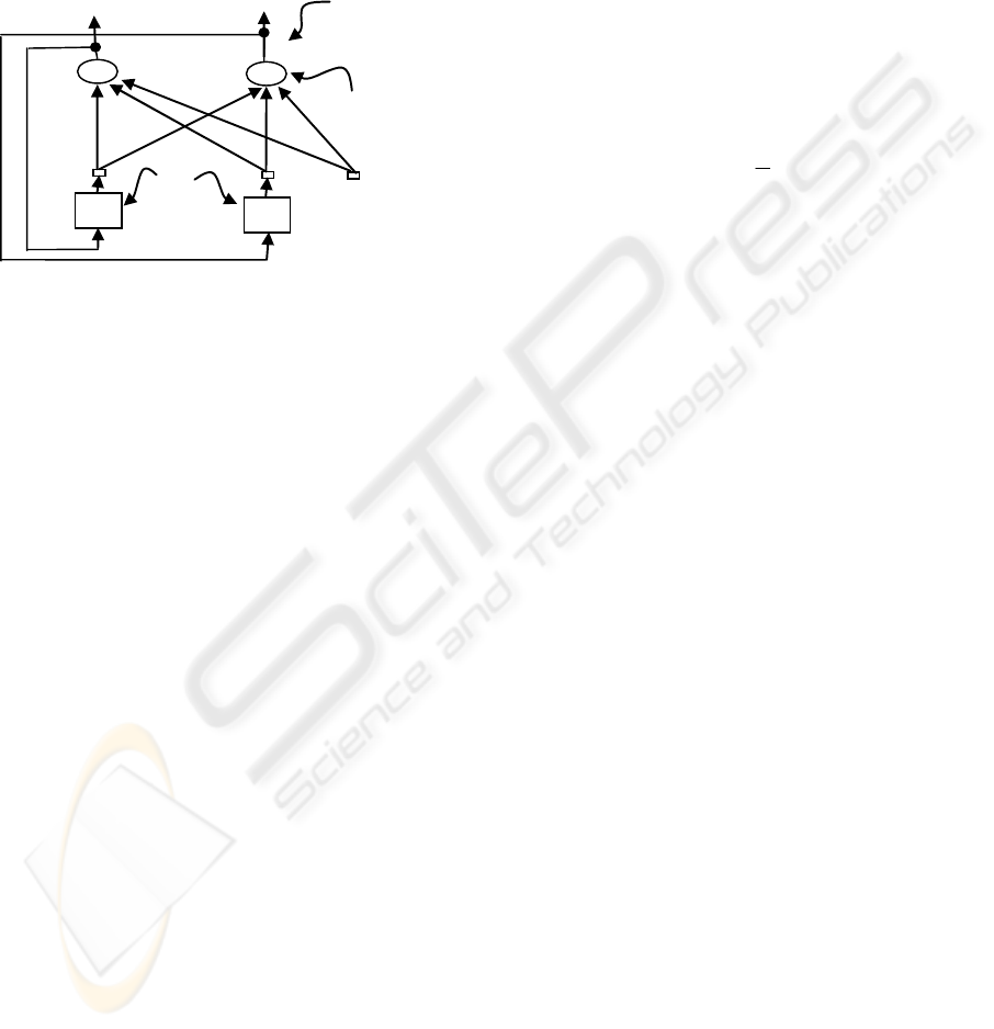
Z
‐1

g
1
:
A
11

A
12

A
21

A
22

B
11

B
21

)1(
~
1
+kx
System
externalinput
Systemdynamics
Systemstate:
internal in
p
ut
Neuron
delay
Z
‐1

Outputs
)(
~
ky
)1(
~
2
+kx

)(
~
1
kx

)(
~
2
kx








Figure 1: A second order recurrent neural network
architecture.
As a general case, consider a network consisting
of a total of N neurons with M external input
connections, as shown in Figure 1 for a 2
nd
model
order. Let the variable g(k) denotes the (M x 1)
external input vector applied to the network at
discrete time k and the variable y(k + 1) denotes the
corresponding (N x 1) vector of individual neuron
outputs produced one step later at time (k + 1). The
input vector g(k) and one-step delayed output vector
y(k) are concatenated to form the ((M + N) x 1)
vector u(k), whose i
th
element is denoted by u
i
(k). If
Λ denotes the set of indices i for which g
i
(k) is an
external input, and β denotes the set of indices i for
which u
i
(k) is the output of a neuron (which is
y
i
(k)), the following is true:
⎪
⎩
⎪
⎨
⎧
∈
∈
β i ,k
y
Λ i ,k
g
= k
u
i
i
i
if)(
if)(
)(
(13)
The (N x (M + N)) recurrent weight matrix of the
network is represented by the variable [W]. The net
internal activity of neuron j at time k is given by:
)()( = )( kukwkv
iji
βΛi
j
∑
∪∈
(14)
At (k + 1), the output of the neuron j is computed by
passing v
j
(k) through the nonlinearity (.)φ :
))((= )1( kvφky
jj
+
(15)
The derivation of the recurrent algorithm maybe
obtained by using d
j
(k) to denote the desired
response of neuron j at time k, and
ς(k) to denote
the set of neurons that are chosen to provide
externally reachable outputs. A time-varying (N x 1)
error vector e(k) is defined whose j
th
element is
given by the following relationship:
⎪
⎩
⎪
⎨
⎧
∈
otherwise 0,
)( if ),( - )(
= )(
kςjkykd
ke
jj
j
(16)
The objective is to minimize the cost function E
total
which is obtained by:
)](
2
1
[)( =
2
total
kekEE
j
ςjkk
∑∑∑
∈
=
(17)
This cost function will be minimized by
estimating the instantaneous gradient, which is the
error at each instant of time k with respect to the
weight matrix [W] and then updating [W] in the
negative direction of this gradient (Haykin, 1994).
As a result:
[
]
]
~
[]
~
[
dd
BAW =
(18)
where
d
A
~
and
d
B
~
are the estimates of Equation (9).
3 SYSTEM TRANSFORMATION
AND ORDER REDUCTION
In the new reduction technique, the system is
transformed before the model order is reduced.
System transformation is achieved by transforming
the system state matrix [A] based on the ANN
estimation and then transforming the [B], [C], and
[D] matrices of Equations (1) and (2) using the LMI-
based transformation.
3.1 ANN System State Matrix
Transformation
In this paper, one objective is to search for a
transformation that decouples different categories of
system eigenvalues. In the transformed system
presented in this paper, the dominant eigenvalue
category is selected as a subset of the original
system eigenvalues. This is accomplished by
transforming the system state matrix [A] in Equation
(1) into [
A
ˆ
] (for all real eigenvalues) as follows:
MODEL-ORDER REDUCTION OF SINGULARLY PERTURBED SYSTEMS BASED ON ARTIFICIAL NEURAL
ESTIMATION AND LMI-BASED TRANSFORMATION
175

⎥
⎥
⎥
⎥
⎦
⎤
⎢
⎢
⎢
⎢
⎣
⎡
=
n
n
n
λ
aλ
aaλ
A
00
0
0
ˆ
22
1121
"
#%#
"
"
(19)
This is an upper triangular matrix that has the
original system eigenvalues preserved in the
diagonal, seen as λ
i
, and has the elements to be
identified, seen as (a
ij
). It is set as such for the
purpose of eliminating the fast dynamics and
sustaining the slow dynamics through model order
reduction. In order to evaluate the (a
ij
) elements,
first, the system of Equations (1) and (2) is
discretized as shown in Equations (9) and (10),
second, the [
d
A ] in Equation (9) is transformed into
[
d
A
~
] (similar to the form seen in Equation (19)),
third, the recurrent neural network estimates the
required elements of [
d
A
~
], fourth, (a
ij
) are then
evaluated once the continuous form is obtained from
the estimated discrete system.
In this estimation, the interest is to estimate or
obtain the [
d
A
~
] only without the estimation of the
[
d
B
~
] matrix, where this [
d
B
~
] matrix is
automatically obtained in the recurrent network as
seen in Figure 1 and Equation (18). In order to
achieve this objective, the zero input (u(k) = 0)
response is obtained where the input/output data is
basically generated based on the initial state
conditions only. Hence, the discrete system of
Equations (9) and (10), with initial state
conditions
0
)0( xx = , becomes:
0
)0( ),()1( xxkxAkx
d
==+
(20)
)()( kxky =
(21)
Now based on Equations (20) and (21), where
the initial states are the system input and the
obtained states are the system output, a set of
input/output data is obtained and the neural network
estimation is applied (Haykin, 1994). In steps:
Step 1. Initialize the weights [W] by a set of
uniformly distributed random numbers. Starting at
the instant k = 0, use Equations (14) and (15) to
compute the output values of the N neurons
(where
ßN = ).
Step 2. For every time step k and all
,ßj ∈ ßm
∈
and
∪∈ ßA Λ, compute the system dynamics which
are governed by the triply indexed set of variables:
⎥
⎥
⎦
⎤
⎢
⎢
⎣
⎡
+=+
∑
∈ßi
mj
i
mjij
j
m
kuδkπkwkvφkπ )()()())(()1(
AA
A

(22)
with initial conditions
0)0( =
j
mA
π
and
mj
δ
given by
(
)
)()( kwkw
mji A
∂
∂
is equal to "1" only when j = m
and
A
=
i ; otherwise it is "0". Notice that for the
special case of a sigmoidal nonlinearity in the form
of a logistic function, the derivative
)(⋅φ

is given by
)]1(1)[1())(( +−+= kykykvφ
jjj

.
Step 3. Compute the weight changes corresponding
to the error signal and system dynamics:
∑
∈
=Δ
ςj
j
m
jm
kπkeηkw )()()(
A
A
(23)
Step 4. Update the weights in accordance with:
)()()1( kwkwkw
mmm AAA
Δ+
=
+
(24)
Step 5. Repeat the above 4 steps for final desired
estimation.
Training the network as illustrated, produces the
discrete transformed system state matrix [
d
A
~
]. This
new discrete matrix is then converted to the
continuous form to give the transformed system state
matrix [
A
ˆ
] as actually seen in Equation (19).
3.2 LMI-based Complete System
Transformation
The transformation in Equation (19) is motivated by
the matrix reducibility concept illustrated as follows
(Boyd, 1994) (Horn, 1985 ):
Definition. A matrix
n
MA
∈
is called reducible if
either:
(a) n = 1 and A = 0; or
(b) n ≥ 2, there is a permutation matrix
n
MP ∈ ,
and some integer r with
11 −≤
≤
nr such that:
⎥
⎦
⎤
⎢
⎣
⎡
=
−
Z
YX
APP
0
1
(25)
where
rr
MX
,
∈
,
rnrn
MZ
−−
∈
,
,
rnr
MY
−
∈
,
, and
0
rrn
M
,−
∈
is a zero matrix.
The attractive features of the permutation matrix
[P] such as being orthogonal and invertible have
made this transformation easy to carry out. Based on
the LMI technique, the optimization problem is
casted as follows:
ICINCO 2009 - 6th International Conference on Informatics in Control, Automation and Robotics
176

o
P
PP −min subject to
εAAPP <−
−
ˆ
1
(26)
which maybe written in an LMI equivalent form as:
)(min Strace
S
subject to
0
)
ˆ
(
ˆ
0
)(
1
12
1
>
⎥
⎥
⎦
⎤
⎢
⎢
⎣
⎡
−
−
>
⎥
⎦
⎤
⎢
⎣
⎡
−
−
−
−
IAAPP
AAPPIε
IPP
PPS
T
T
o
o
(27)
where S is a symmetric slack matrix (Boyd, 1994).
The Linear Matrix Inequalities (LMI) are applied
to the [
A] and [ A
ˆ
] matrices and the transformation
matrix [
P] is then obtained, which is necessary for
obtaining the complete system transformation {[
B
ˆ
],
[
C
ˆ
], [
D
ˆ
]}. Complete system transformation can be
achieved as follows: assuming that
xPx
1
ˆ
−
= , the
system of Equations (1) and (2) can be re-written as:
)()(
ˆ
)(
ˆ
tButxAPtxP +=

(28)
)()(
ˆ
)(
ˆ
tDutxCPty
+
=
(29)
Pre-multiplying Equation (28) by [P
-1
] yields:
)(
ˆ
)(
ˆ
ˆ
)(
ˆ
)()(
ˆ
)(
ˆ
111
tuBtxAtx
tBuPtxAPPtxPP
+=∴
+=
−−−


(30)
)(
ˆ
)(
ˆ
ˆ
)(
ˆ
)()(
ˆ
)(
ˆ
and
tuDtxCty
tDutxCPty
+=∴
+=
(31)
where the transformed system matrices are:
AP
P
A
1
ˆ
−
= ,
B
P
B
1
ˆ
−
=
,
CPC =
ˆ
, and
D
D
=
ˆ
.
3.3 Model Order Reduction
Model order reduction will now be applied to the
system of Equations (30) and (31) which has the
following format:
)(
)(
ˆ
)(
ˆ
0
)(
ˆ
)(
ˆ
tu
B
B
tx
tx
A
AA
tx
tx
o
r
o
r
o
crn
o
r
⎥
⎦
⎤
⎢
⎣
⎡
+
⎥
⎦
⎤
⎢
⎣
⎡
⎥
⎦
⎤
⎢
⎣
⎡
=
⎥
⎥
⎦
⎤
⎢
⎢
⎣
⎡


(32)
[]
)(
ˆ
)(
ˆ
)(
ˆ
)(
ˆ
tuD
tx
tx
CCty
o
r
orn
+
⎥
⎦
⎤
⎢
⎣
⎡
=
(33)
Notice that in the new formulation, the dominant
eigenvalues (slow dynamics) which are presented
in
rn
A are now decoupled from the non-dominant
eigenvalues (fast dynamics) which are presented
in
o
A . Hence, as illustrated in Equations (3) and (4)
for order reduction, Equation (32) is written as:
)()(
ˆ
)(
ˆ
)(
ˆ
tuBtxAtxAtx
rocrrnr
++=

(34)
)()(
ˆ
)(
ˆ
tuBtxAtx
oooo
+=

(35)
By neglecting the system fast dynamics
(setting
)(
ˆ
tx
o

= 0 by setting 0=ε )), the coupling
term
)(
ˆ
txA
oc
is evaluated by solving for )(
ˆ
tx
o
in
Equation (35). That is,
)()(
ˆ
1
tuBAtx
ooo
−
−= and the
reduced model order becomes:
)(][)(
ˆ
)(
ˆ
1
tuBBAAtxAtx
roocrrnr
+−+=
−

(36)
)(][)(
ˆ
)(
ˆ
1
tuDBACtxCty
ooorr
+−+=
−
(37)
Hence, the overall transformed reduced model order
is given by:
)()(
ˆ
)(
ˆ
tuBtxAtx
orrorr
+=

(38)
)()(
ˆ
)(
ˆ
tuDtxCty
orror
+
=
(39)
where the details of the {[
or
A ], [
or
B ], [
or
C ],
[
or
D ]} overall reduced matrices are shown in
Equations (36) and (37).
4 SIMULATIONS AND RESULTS
The proposed method of reduced order system
modeling based on neural network estimation, LMI-
based transformation, and model order reduction is
investigated the following case studies.
Case Study. Consider the system of a high-
performance tape transport shown in Figure 2
(Franklin, 1994). The system is designed with a
small capstan to pull the tape past the read/write
heads with the take-up reels turned by DC motors. In
the static equilibrium, the tape tension equals the
vacuum force
FT
o
=
and the torque from the motor
equals the torque on the capstan
oot
TriK
1
= . Please
notice that all the variables are defined in (Franklin,
1994).
MODEL-ORDER REDUCTION OF SINGULARLY PERTURBED SYSTEMS BASED ON ARTIFICIAL NEURAL
ESTIMATION AND LMI-BASED TRANSFORMATION
177

Figure 2: Tape-drive system schematic control model.
The variables are defined as deviations from the
equilibrium. The system equations of motion are
given as follows:
iKTrωβ
d
t
ωd
J
t
+−+=
111
1
1
,
111
ωrx =

eωKRi
d
t
di
L
e
=+
1
,
222
ωrx =

0
222
2
2
=++ Trωβ
d
t
ωd
J
)()(
131131
xxDxxKT

−+−=
)()(
322322
xxDxxKT

−
+
−=
111
θrx = ,
222
θrx = ,
2
21
3
xx
x
−
=
,
The state space model is derived from the system
equations, where there are (i) one input, which is the
applied voltage, (ii) three outputs, which are: (1)
tape position at the head, (2) tape tension, and (3)
tape position at the wheel, (iii) five states: (1) tape
position at the air bearing, (2) drive wheel speed, (3)
tape position at the wheel, (4) tachometer output
speed, and (5) capstan motor speed. For dynamical
testing of the new reduction technique validity,
different cases of this practical system were
investigated.
As a first example, a system with all real
eigenvalues is considered:
)(
1
0
0
0
0
)(
10-000.03-0
05.4-1.4-0.40.35
05000
0.7504.10.11.35-0.1-
00020
)( tutxtx
⎥
⎥
⎥
⎥
⎥
⎥
⎦
⎤
⎢
⎢
⎢
⎢
⎢
⎢
⎣
⎡
+
⎥
⎥
⎥
⎥
⎥
⎥
⎦
⎤
⎢
⎢
⎢
⎢
⎢
⎢
⎣
⎡
=

)(
02.02.02.02.0
005.005.0
00100
)( txty
⎥
⎥
⎥
⎦
⎤
⎢
⎢
⎢
⎣
⎡
−−
=
with the eigenvalues {-9.9973, -3.9702, -1.8992,
-0.677, -0.2055}. Since there are two categories of
eigenvalues, slow {-1.8992, -0.6778, -0.2055} and
fast {-9.9973, -3.9702}, model order reduction may
be applied.
Discretizing this system with a sampling period
T
s
= 0.1s, simulating the discrete system for 200
input/output data points, and training it with learning
rate of
η = 1 x 10
-4
and initial weights for ]
~
[
d
A :
⎥
⎥
⎥
⎥
⎥
⎥
⎦
⎤
⎢
⎢
⎢
⎢
⎢
⎢
⎣
⎡
=
0.0121 0.0049 0.0091 0.0024 0.0102
0.0051 0.0076 0.0078 0.0039 0.0055
0.0034 0.0175 0.0136 0.0176 0.0176
0.0040 0.0017 0.0048 0.0024 0.0072
0.0168 0.0089 0.0009 0.0039 0.0048
w
produces the transformed system matrix:
⎥
⎥
⎥
⎥
⎥
⎥
⎦
⎤
⎢
⎢
⎢
⎢
⎢
⎢
⎣
⎡
=
9.9963-0000
0.09203.9708-000
0.05370.22821.8986-00
0.05540.01560.05130.6782-0
0.20740.07620.0068-0.0367-0.2051-
ˆ
A
with estimated eigenvalues -9.9963, -3.9708, -1.898,
-0.6782, -0.2051. This was achieved by decoupling
the fast eigenvalue category from the slow one,
which simply was done by first placing the slow
eigenvalue category in
λ
i
of Equation (19) and then
the fast category. As observed in
A
ˆ
above, the
eigenvalues are almost identical with the original
system with little difference due to discretization.
Using the LMI-based system transformation, the
complete transformed system is obtained.
Considering the {-9.9963, -3.9708} as the fast
category eigenvalue, the 3
rd
order reduced model is
determined. Simulation results based on (i) model
order reduction without system transformation, (ii)
model order reduction with ANN transformation
(estimation of
]
~
[
d
A and ]
~
[
d
B matrices only as
presented in Equations (11) and (12)), (iii) model
order reduction with LMI-based complete system
transformation, and (iv) the original 5
th
order system
are all shown in Figure 3.
ICINCO 2009 - 6th International Conference on Informatics in Control, Automation and Robotics
178

0 5 10 15 20 25 30 35 40
-0.2
-0.1
0
0.1
0.2
0.3
0.4
0.5
0.6
0.7
___ Original, ---- Trans. with LMI, -.-.- None Trans., .... Trans. without LMI
Tim e[ s]
System Output
Y1
Y2
Y3
Figure 3: Reduced 3
rd
model orders (Pink.…. transformed
with ANN estimation only, Red-.-.-.- non-transformed,
Black---- transformed with LMI) output responses to a
step input along with the non reduced (Blue____ original)
system output response. The LMI-transformed curve fits
almost exactly on the original response.
For more rigorous testing of the new reduction
technique, the 5
th
model order is reduced to a 2
nd
order assuming that the -1.8986 belongs to the fast
eigenvalue category. Hence, the 2
nd
order reduced
model with its eigenvalues preserved as desired is
obtained:
)(
2.1764-
1.9672-
)(
ˆ
0.6782-0
0.0367-0.2051-
)(
ˆ
tutxtx
rr
⎥
⎦
⎤
⎢
⎣
⎡
+
⎥
⎦
⎤
⎢
⎣
⎡
=

)(
0.0005
0.0043
0.0018
)(
ˆ
0.0140-0.0217
0.10290.1055-
0.04510.0436-
)(
ˆ
tutxty
r
⎥
⎥
⎥
⎦
⎤
⎢
⎢
⎢
⎣
⎡
+
⎥
⎥
⎥
⎦
⎤
⎢
⎢
⎢
⎣
⎡
=
Simulating this reduced 2
nd
model order as
performed for the 3
rd
model order, provided the
results shown in Figure 4 where the new reduction
technique results in responses are identical to the
original system's.
As a second example, the system considered here
consists of two complex eigenvalues and three real,
0 5 10 15 20 25 30 35 40
-0.2
-0.1
0
0.1
0.2
0.3
0.4
0.5
0.6
0.7
___ Original, ---- Trans. with LMI, -.-.- None Trans., .... Trans. without LMI
Time[s ]
System Output
Y1
Y2
Y3
Figure 4: Plots of Pink…. 3
rd
order transformed with ANN
estimation only and reduced 2
nd
model orders (Red-.-.-.-
non-transformed, Black---- transformed with LMI) output
responses to a step input along with the non reduced
(Blue____ original) system output response. The LMI-
transformed curve fits almost exactly on the original
response.
where two of the real eigenvalues produce fast
dynamics. The system is given by:
)(
1
0
0
0
0
)(
10-000.03-0
011.4-2.4-1.41.35
05000
0.753.11.11.35-1.1-
00020
)( tutxtx
⎥
⎥
⎥
⎥
⎥
⎥
⎦
⎤
⎢
⎢
⎢
⎢
⎢
⎢
⎣
⎡
+
⎥
⎥
⎥
⎥
⎥
⎥
⎦
⎤
⎢
⎢
⎢
⎢
⎢
⎢
⎣
⎡
=

,
)(
02.02.02.02.0
005.005.0
00100
)( txty
⎥
⎥
⎥
⎦
⎤
⎢
⎢
⎢
⎣
⎡
−−
=
The five eigenvalues are {-10.5772, -9.999, -0.9814,
-0.5962 ± j0.8702}. Considering the {-10.5772,
-9.999} as the fast eigenvalue category, model order
reduction is performed.
Discretizing the system with
T
s
= 0.1s, using a
step input with a learning time
T
l
= 15s, and training
the ANN for the input/output data with
η = 0.001
learning rate produces the transformed system
matrix:
⎥
⎥
⎥
⎥
⎥
⎥
⎦
⎤
⎢
⎢
⎢
⎢
⎢
⎢
⎣
⎡
=
10.5764-0000
1.0449 9.9985-000
0.49340.13950.9809-00
0.21140.61650.22760.5967-0.8701-
0.0964-0.9860-1.46330.8701-0.5967
ˆ
A
MODEL-ORDER REDUCTION OF SINGULARLY PERTURBED SYSTEMS BASED ON ARTIFICIAL NEURAL
ESTIMATION AND LMI-BASED TRANSFORMATION
179

As observed, all the system eigenvalues have
been preserved. Based on this transformed matrix,
using the LMI technique, the permutation matrix [P]
is computed and then used for obtaining the [
B
ˆ
],
[
C
ˆ
], and [ D
ˆ
] matrices. Since there are two
eigenvalues that produce fast dynamics, the
following 3
rd
order reduced model is obtained:
)(
4.1652-
47.3374-
35.1670
)(
ˆ
0.9809-00
0.22760.5967-0.8701-
1.4633-0.87010.5967-
)(
ˆ
tutxtx
rr
⎥
⎥
⎥
⎦
⎤
⎢
⎢
⎢
⎣
⎡
+
⎥
⎥
⎥
⎦
⎤
⎢
⎢
⎢
⎣
⎡
=

)(
0.0006
0.0025-
0.0025-
)(
ˆ
0.0021-0.0004 0.0001-
0.0088-0.0009-0.0024-
0.0139-00.0019-
)(
ˆ
tutxty
r
⎥
⎥
⎥
⎦
⎤
⎢
⎢
⎢
⎣
⎡
+
⎥
⎥
⎥
⎦
⎤
⎢
⎢
⎢
⎣
⎡
=
The reduced model has also preserved the original
system dominant eigenvalues {-0.9809, -0.5967±
j0.8701}, which achieves the proposed objective.
Investigating the performance of this reduced model
order compared with the other reduction techniques
shows again its superiority as seen in Figure 5. The
LMI-based transformed responses are almost
identical to the 5
th
order original systems'.
0 1 2 3 4 5 6 7 8
-0.02
0
0.02
0.04
0.06
0.08
0.1
0.12
0.14
___ Original, ---- Trans. with LMI, -.-.- None Trans., .... Trans. without LMI
Tim e[ s ]
System Output
Y1
Y2
Y3
Figure 5: Reduced 3
rd
model orders (Pink…. transformed
with ANN estimation only, Red-.-.-.- non-transformed,
Black---- complete transformation with LMI) output
responses to a step input along with the non reduced
(Blue____ original) system output response. The LMI-
transformed curve fits almost exactly on the original
response.
5 CONCLUSIONS
In this paper, a new method of dynamic systems
model order reduction is presented that has the
following advantages. First, in the transformed
model, a decoupling of the slow and fast dynamics is
achieved. Second, in the reduced model order, the
eigenvalues are preserved as a subset of the original
system. Third, the reduced model order shows
responses that are usually almost identical to the
original full order system. Hence, observing the
simulation results, it is clear that modeling of
dynamic systems using the new LMI-based
reduction technique is superior to those other
reduction techniques.
REFERENCES
Alsmadi, O., Abdalla, M., 2007. Model order Reduction
for Two-Time-Scale Systems Based on Neural
Network Estimation. Proceedings of the 15
th
Mediterranean Conference on Control & Automation.
Athens, Greece.
Benner, P., 2007. Model Reduction at ICIAM'07. SIAM
News, V. 40, N. 8.
Boyd, S., El Ghaoui, L., Feron, E., Balakrishnan, V.,
1994. Linear Matrix Inequalities in System and
Control Theory. Society for Industrial and Applied
Mathematics (SIAM).
Bui-Thanh, T., Willcox, K., 2005. Model Reduction for
Large-Scale CFD Applications using the Balanced
Proper Orthogonal Decomposition. 17
th
American
Institute of Aeronautics and Astronautics
Computational Fluid Dynamics Conference. Toronto,
Canada.
Franklin, G., Powell, J., Emami-Naeini, A., 1994.
Feedback Control of Dynamic Systems, Addison-
Wesley, 3
rd
edition.
Garsia, G., Dfouz, J., Benussou, J., 1998. H2 Guaranteed
Cost Control for Singularly Perturbed Uncertain
Systems. IEEE Transactions on Automatic Control,
Vol. 43, pp. 1323-1329.
Haykin, S., 1994. Neural Networks: a Comprehensive
Foundation, Macmillan College Publishing Company,
New York.
Hinton, G., Salakhutdinov, R., 2006. Reducing the
Dimensionality of Data with Neural Networks.
Science, pp. 504-507.
Horn, R., Johnson, C., 1985. Matrix Analysis. Cambridge,
UK.
Kokotovic, P., Khalil, H., O'Reilly, J., 1986. Singular
Perturbation Methods in Control: Analysis and
Design, Academic Press. Orlando, Florida.
Williams, R., Zipser, D., 1989. A Learning Algorithm for
Continually Running Full Recurrent Neural Networks.
Neural Computation, 1(2), pp. 270-280.
Zhou, W., Shao, S., Gao, Z., 2009. A Stability Study of
the Active Disturbance Rejection Control Problem by
a Singular Perturbation Approach. Applied
Mathematical Science, Vol. 3, no. 10, pp. 491-508.
Zurada, J., 1992. Artificial Neural Systems, West
Publishing Company, New York.
ICINCO 2009 - 6th International Conference on Informatics in Control, Automation and Robotics
180