
FIXED POINT SVD COMPUTATION ERROR
CHARACTERIZATION AND PERFORMANCE LOSSSES IN
MIMO SYSTEMS
César Benavente-Peces
1
, Andreas Ahrens
2
1
Universidad Politécnica de Madrid, EUIT Telecomunicación, Ctra. Valencia. km. 7, 28031 Madrid, Spain
2
Hochschule Wismar, University of Technology, Business and Design, Philipp-Müller-Straße 14, 23966 Wismar, Germany
José M. Pardo-Martín, Fco. Javier Ortega-González
Universidad Politécnica de Madrid, EUIT Telecomunicación, Ctra. Valencia. km. 7, 28031 Madrid, Spain
Keywords: Multiple Input Multiple Output (MIMO) systems, Singular Value Decomposition (SVD), Bit Allocation,
Power Allocation, Wireless Transmission, Finite Word Length, Fixed Point Arithmetic.
Abstract: This paper is devoted to analyze the error met when computing the singular value decomposition (SVD) of
the gain channel matrix in a MIMO communication system and using fixed-point arithmetic for the
calculations. The study is focused in the case of the SVD implementation for modulation-mode and power
assignment in non-frequency selective MIMO, and M-ary Quadrature Amplitude Modulation (QAM). It is
demonstrated that not necessarily all MIMO layers must be activated. The combination of the CORDIC
algorithm and look-up tables seems to be a good solution for this task since it can efficiently compute the
singular value decomposition. The paper highlights the characterization of computation errors and shows
the performance losses produced by the use of approximations in the eigenvalues and eigenvectors
calculation, including the effects produced in the power assignment process.
1 INTRODUCTION
MIMO technology has attracted a lot of attention in
wireless systems, since it offers significant increases
in data transmission rate and link range without the
need of providing larger bandwidths or transmitted
power, and a significant BER improvement. The
main goal of MIMO techniques is achieving higher
spectral efficiency and increased reliability. The
application of such techniques involves the
appropriate data processing to obtain their expected
advantages and can be considered as an essential
part of increasing both the achievable capacity and
integrity of future generations of wireless
communication systems (Kühn, 2006), (Zheng and
Tse, 2003).
The SVD performs an estimation of the
eigenvalues and eigenvectors of the gains channel
matrix. It allows transforming a MIMO channel into
multiple single input single output (SISO) channels
having unequal gains.
In order to avoid any signalling overhead, fixed
transmission modes are investigated in (Ahrens and
Lange, 2008) regardless of the channel quality. The
study’s results have shown that not all MIMO layers
have to be activated in order to achieve the best bit
error rate.
Assuming perfect channel state information
(PCSI), the channel capacity can only be achieved
by using water-pouring procedures. However, in
practical application only finite and discrete
transmission rates are possible. Therefore, in this
contribution the efficiency of fixed transmission
modes is studied regardless of the channel quality.
Furthermore, this paper focuses on the analysis
of the error met when computing the SVD of the
gain channel matrix in a MIMO system and using
finite word length and fixed point arithmetic,
specifically for modulation-mode and power
assignment, using computationally efficient
algorithms.
The paper remarks the feasibility of using
appropriate approximations to implement the SVD
91
Benavente-Peces C., Ahrens A., M. Pardo-Martín J. and Javier Ortega-González F. (2009).
FIXED POINT SVD COMPUTATION ERROR CHARACTERIZATION AND PERFORMANCE LOSSSES IN MIMO SYSTEMS.
In Proceedings of the International Conference on Wireless Information Networks and Systems, pages 91-94
DOI: 10.5220/0002188800910094
Copyright
c
SciTePress
providing low computational load operations with
small performance degradation, focusing on MIMO
channels using M-ary QAM.
2 SYTEM MODEL DESCRIPTION
We consider a single MIMO system with PCSI at
both the transmission and reception sides. We model
the channel as a flat independent and identically
distributed (i.i.d.) Rayleigh channel. Given a MIMO
system with n
T
aerials at the transmitter and n
R
at the
receiver, the received signal can be expressed as
y=H•s+n, (1)
where y is the n
R
×
1 sized received signal vector, s is
the n
T
×
1 transmitted signal vector containing the
complex input symbols and n is the n
R
×
1 vector of
the additive white Gaussian noise (AWGN) with
variance var(Re[n
R
]) = var(Im[n
R
]) = σ
2
/2.
H is the n
R
×
n
T
complex channel gain matrix with
entries also having unit magnitude variance. We
assume that n
T
equals n
R
. In order to convert the
MIMO system into several SISO channels, data
vector s is multiplied by the matrix V before
transmission. The received signal is preprocessed by
multipling it by the matrix U
H
to obtain the received
data vector
y
ˆ
.
0
0,1
0,2
0,3
0,4
0,5
0,6
0,7
0,8
0,9
1
0
,0
2
0
,0
6
0
,1
0
0
,1
4
0
,1
8
0
,2
2
0
,2
6
0
,3
0
0
,3
4
0
,3
8
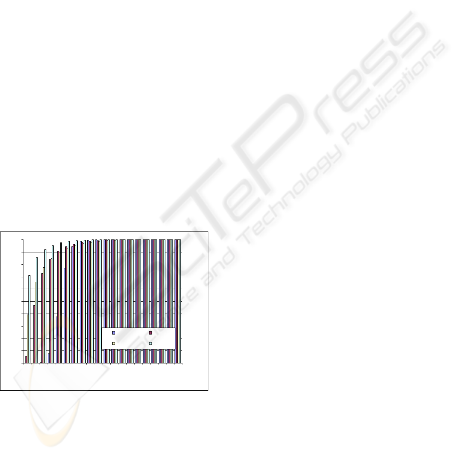
error bound
Probability of meeting an error up to the bou
Coef 1 Coef 2
Coef 3 Coef 4
Figure 1: Probability of getting eigenvalues a magnitude
error up to defined values, for n
T
=n
R
=4 MIMO case.
3 THE SVD PRINCIPLES
The SVD of a real n
R
×
n
T
matrix H means factorizing
into the product of three matrices,
H =UΣV
H
, (2)
where U and V are orthogonal n
R
×
n
T
unitary
matrices and Σ = diag(σ
1
,σ
2
,...,σ
n
) is an n
R
×
n
T
diagonal matrix containing the singular values of H,
where n equals min(n
R
,n
T
). The columns of U and V
are called respectively the left and right singular
vectors and σ
i
the ith singular value of H. Within this
work, we assume that n
T
equals n
R
, i.e., H is
assumed to be a non-singular square matrix.
4 FUNDAMENTALS OF THE
CORDIC ALGORITHM
The CORDIC (COordinate Rotation Digital
Computer) algorithm consists of an iterative
algorithm that allows computing relatively complex
functions by using simple operations, just addition
and shift operations.
In the most general form, a CORDIC algorithm
iteration used to perform a rotation is described by:
z(k+1)=z(k)-
σ
·atan(2
-
k
),
x(k+1)=x(k)-y(k)·
σ
·(2
-k
),
y(k+1)=y(k)+x(k) · σ·(2
-k
),
(3)
where k ranges from 0 to N, being N the number of
iterations, and
σ
takes the value +1 if z(k) is equal
or greater than 0 and –1 otherwise, and the samples x
and y correspond to the coordinates. The target angle
equals z(0). Phase micro-rotations are determined by
z that is forced to become zero in the iterative
process. The application of the CORDIC algorithm
using (3) has the immediate advantage that it does
not require product units. Some efficient strategy
must be used to compute the atan function.
Authors present more details on the
implementation of the singular value decomposition
using finite word length and fixed-point arithmetic
in (Benavente-Peces et al., 2008).
5 ERROR DESCRIPTION AND
ANALYSIS
This section analyses the error computing eigenvalus
eith fixed point arithmetic to predict system
performance and degradation. As an example we
have considered a 4x4 (four transmitting and four
receiving antennas) MIMO system and the channel
is modeled as a flat independent and identically
distributed (i.i.d.) Rayleigh one.
WINSYS 2009 - International Conference on Wireless Information Networks and Systems
92
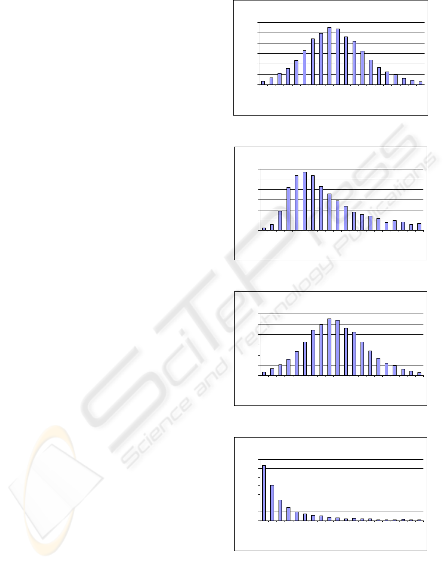
Figure 1 shows the computation of the
probability of getting the eigenvalues an error up to
a predefined bound. Eigenvalues are arranged from
largest to smallest as Coef 1 to Coef 4. If we take
into acount that eigenvectors are arranged in
decreasing order, it is noticable that lower values are
affected by larger errors.
The eigenvalues were computed using the Jacobi
method and the CORDIC algorithm was applied
with 16-bits. The main conclusion is that power
allocation will be affected by the erros in the
eigenvalues computation and degrading the system
performance.
The Jacobi iterations search for largest off-
diagonal element in H and eliminates it by rotations,
finding one eigenvalue. So, the largest eigenvalue is
obtained at first, being affected by smaller errors.
Fortunately, the largest eigenvalue is the most
influencing in the transmission, producing a lower
effect on the performance degradation.
Figures 2 to 5 show the error probability
distribution met for each eigenvalue (Coef 1 to Coef
4) in the interval we obtain the more significant
values.
The distribution of errors for “Coef 1” and “Coef
3” seem to follow a gaussain distribution with the
mean given by the mean value of the computation
error.
On the other hand, the errors for “Coef 2” and
“Coef 4” are far a way from a gaussian distribution.
In the case of “Coef 2”, it could be considered as a
gaussian distribution in a narrow interval due to the
assimetry. Errors in “Coef 4” eigenvalue looks an
exponential distribution function.
This behaviour suggests the possibility of
modelling the computation of the eigenvalues as the
given value disturbed by noise that could be
approximated by a gaussian distribution. It allows
the prediction of the system performance.
6 QUALITY CRITERIA
There are two possibilities, one based on the
measurement of the channel capacity and compare
the results to the traditional SISO (single input
single output) system, and other based on the BER
measurement obtained for various SNR and compare
the gain of the MIMO system using full precision in
SVD computation to the SISO case.
Coef 1
0
0,02
0,04
0,06
0,08
0,1
0,12
0,0600
0,0650
0,0700
0,0750
0,0800
0,0850
0,0900
0,0950
0,1000
0,1050
0,1100
0,1150
0,1200
0,1250
0,1300
0,1350
0,1400
0,1450
0,1500
0,1550
Values
Probabilit
y
Figure 2: Probability error distribution for Coef 1.
Coef 2
0
0,02
0,04
0,06
0,08
0,1
0,12
0,0050
0,0100
0,0150
0,0200
0,0250
0,0300
0,0350
0,0400
0,0450
0,0500
0,0550
0,0600
0,0650
0,0700
0,0750
0,0800
0,0850
0,0900
0,0950
0,1000
Values
Probabilit
y
Figure 3: Probability error distribution for Coef 2.
Coef 3
0
0,02
0,04
0,06
0,08
0,1
0,12
0,0000
0,0050
0,0100
0,0150
0,0200
0,0250
0,0300
0,0350
0,0400
0,0450
0,0500
0,0550
0,0600
0,0650
0,0700
0,0750
0,0800
0,0850
0,0900
0,0950
Values
Probabilit
y
Figure 4: Probability error distribution for Coef 3.
Coef 4
0
0,05
0,1
0,15
0,2
0,25
0,3
0,35
0,0000
0,0050
0,0100
0,0150
0,0200
0,0250
0,0300
0,0350
0,0400
0,0450
0,0500
0,0550
0,0600
0,0650
0,0700
0,0750
0,0800
0,0850
0,0900
0,0950
Values
Probabilit
y
Figure 5: Probability error distribution for Coef 4.
6.1 Channel capacity
Figure 6 shows the channel capacity of the MIMO
FIXED POINT SVD COMPUTATION ERROR CHARACTERIZATION AND PERFORMANCE LOSSSES IN MIMO
SYSTEMS
93
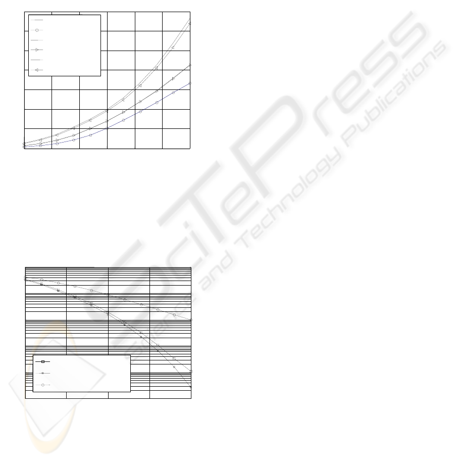
channel for various n
T
and n
R
combinations. The
unmarked line corresponds to SVD full precision
computation. Marked lines correspond to the MIMO
channel capacity computed using the CODIC with
fixed point arithmetic. As consequence of the errors,
the power is not allocated appropriately provocating
capacity losses. These effects are more remarkable
for larger signal to noise ratios where computation
noise is more noticiable. Besides, those errors are
large for larger number of antennas.
-10
-5
0
5
10
15
20
0
2
4
6
8
10
12
14
SND (dB)
Capacity (bps/Hz)
n
T
=n
R
=1
n
T
=n
R
=1 (fixed point)
n
T
=n
R
=2
n
T
=n
R
=2 (fixed point)
n
T
=n
R
=4
n
T
=n
R
=4 (fixed point)
Figure 6: Channel capacity.
6.2 Bit Error Rate
In general, the quality can be informally assessed by
using the (SNR) at the detector’s (Ahrens and
Lange, 2007).
0
5
10
15
20
10
-5
10
-4
10
-3
10
-2
10
-1
10
0
Eb/No (dB)
BER
n
T
=n
R
=4 (finite precision)
n
T
=n
R
=4 (full precision)
n
T
=n
R
=1
Figure 7: BER comparison for the case n
T
=n
R
=4.
Figure 7 shows the BER for various signal to
noise ratios. QAM is used on all activated MIMO
layers. In the figure we compare the results obtained
using full precision with those obtained when using
the CORDIC with finite word length and fixed point
arithmetic to compute the SVD and these values are
used to analyse the MIMO system performance.
7 CONCLUSIONS
The work reveals that larger errors are found for the
smaller eigenvalues. This is due to the Jacobi
algorithm application to perform the SVD
decomposition using the CORDIC iterations. We
conclude that the largest singular values are quite
robust against computation errors and vice verse.
Finite word length and fixed point arithmetic
decreases system capacity. The loss results very
little when using 16 bits for SVD computation and
data processing. From the point of view of the BER,
the use of finite word length and fixed point
arithmetic increases the BER in relation to the full
precision implementation. For 16-bits arithmetic the
losses are moderate. The combined use of the
CORDIC algorithm and look-up tables for
computing the SVD of H in a non-frequency
selective MIMO system applying the Jacobi
algorithm and using fixed point arithmetic provides
a very efficient tool with very low computational
load and complexity with acceptable losses in the
system performance.
REFERENCES
Kühn, V., 2006. Wireless Communications over MIMO
Channels – Applications to CDMA and Multiple
Antenna Systems. Chichester: Wiley.
Zheng, L. and Tse, D. N. T., 2003. “Diversity and
Multiplexing: A Fundamental Tradeoff in Multiple-
Antenna Channels”, IEEE Transactions on
Information Theory, vol. 49, no. 5, pp. 1073–1096,
May.
Ahrens, A. and Lange, C., 2008. “Modulation-Mode and
Power Assignment in SVD-equalized MIMO
Systems.” Facta Universitatis (Series Electronics and
Energetics), vol. 21, no. 2, pp. 167–181, August.
Benavente-Peces, C., Ahrens, A., Arriero-Encinas, L. and
Lange, C., 2008 ”Implementation Analysis of SVD for
Modulation-Mode and Power Assignment in MIMO
Systems”, 7th IASTED International Conference on
Communications Systems and Networks (CSN),
Palma de Mallorca ( Spain), 01-03 September.
Ahrens, A. and Lange, C., 2007. Transmit Power
Allocation in SVD Equalized Multicarrier Systems,
International Journal of Electronics and
Communications (AEÜ), 61 (1), pp 51–61.
WINSYS 2009 - International Conference on Wireless Information Networks and Systems
94
