THEORETICAL CALCULATION OF THERMAL CONTACT
RESISTANCE OF BALL BEARING UNDER DIFFERENT LOADS
Chao Jin, Bo Wu
State Key Laboratory for Digital Manufacturing Equipment and Technology
Huazhong University of Science and Technology, Wuhan, Hubei 430074, China
Youmin Hu
School of Mechanical Science and Engineering, Huazhong University of Science and Technology
Keywords: Hertzian theory, JHM method, Load distribution, Thermal contact resistance.
Abstract: The thermal contact resistance between the balls and the inner and outer rings of an angular contact ball
bearing is investigated. It is assumed that the bearing sustains thrust, radial, or combined loads under a
steady-state temperature condition. The shapes and sizes of the contact areas are calculated using the
Hertzian theory. The distribution of internal loading in the bearing is determined by the JHM method. The
comparison between the experimental data and the calculated values confirms the validity of the prediction
method for the thermal contact resistances between the elements of a bearing.
1 INTRODUCTION
In a high-speed feeding system, bearings are
considered to be the main heat sources, and the
thermal properties of the bearings need to be
carefully studied. For a bearing, the thermal
resistances for conduction through the bearing
elements themselves and for radiation can be
calculated using the dimensions, the thermal
conductivities, the thermal-optical properties, and
the temperatures of the elements. However, it ca be
said that the thermal contact resistances between the
balls and the rings, which are most closely related to
the temperature differences across the bearings, are
difficult to predict because few useful calculation
method have been proposed yet.
Since the thermal resistance results from the fact
that most of the heat is constrained to flow through
small contact areas, a reasonable step in determining
the contact resistance between the balls and the inner
and outer rings of the bearing would be to use a
similar approach to that adopted to solve the thermal
constriction problem for ideal smooth surfaces. The
thermal constriction resistances for circular, circular
annular, rectangular, and other geometrical-shaped
contact areas are normally solved analytically or
numerically as Dirichlet problems. The prediction of
the thermal contact resistance necessitates the
determination of the contact area. This is possible
with the Hertzian theory when the contact surfaces
are approximated as being smooth. In addition to the
study by Clausing and Chao, the thermal contact
resistance problem has been discussed in many
papers. Most papers determine the contact areas
using the Hertzian theory. However, a survey of the
literature shows that only the studies by Yovanovich
have dealt with the problem of the contact resistance
between bearing elements. He studied the contact
resistance under axial loads and concluded that the
contact resistance depends on the size and shape of
contact area as determined by the Hertzian theory
and the thermal conductivity of the material. He did
not, however, give thermal designers a tractable
expression that considered the change in contact
angle induced by elastic deformation at the contact
points. Also, he did not consider other types of
loadings such as radial and combined axial/radial
loads.
This article develops an approach that accurately
predicts the thermal contact resistance between the
balls and the inner and outer rings of an angular
contact ball bearing. The contact forces required to
calculate the contact area are explicitly formulated
for axial, radial, and combined loadings. The
prediction method for the thermal contact resistance
is verified by comparing the calculated values with
181
Jin C., Wu B. and Hu Y. (2009).
THEORETICAL CALCULATION OF THERMAL CONTACT RESISTANCE OF BALL BEARING UNDER DIFFERENT LOADS.
In Proceedings of the 6th International Conference on Informatics in Control, Automation and Robotics - Intelligent Control Systems and Optimization,
pages 181-188
DOI: 10.5220/0002192401810188
Copyright
c
 SciTePress

experimental results measured in a high-speed
feeding system.
2 EXPRESSIONS FOR CONTACT
RESISTANCE
2.1 Contact Resistance
The contact resistances between the balls and the
inner and outer rings may be treated in the same
manner as constriction resistance since both
resistances result from the restriction of the heat
flow due to small contact arrears. Thus, the
assumptions utilized to solve the constriction
resistance may be applicable to the present problem.
It is assumed that one half of the thermal
constriction resistance problem can be adequately
represented by an isolated, isothermal area either
supplying or receiving heat from an other-wise
insulated conducting half-space. In the ellipsoidal
coordinate system the Laplace’s equation is:
))((
2
u
T
uf
u
T
∂
∂
∂
∂
∇ ＝
(1)
Where
uubuauf ))(()(
22
++=
(2)
And a, b are the semi-major and semi-minor axes
of the elliptic contact area, respectively; while u is
the variable along an axis normal to the contact
plane. The boundary conditions are:
0
,0 TTu == , const
0, =∞→ Tu
(3)
(4)
With Equation (1), (3) and (4), the temperature
distribution can be obtained:
∫
∞
=
u
uf
du
k
Q
T
)(
4
π
(5)
Where Q is all the heat leaving the elliptic
contact area, and by the definition of the thermal
contact resistance:
∫
∞
∞→
=
−
=
0
0
)(
4
1
uf
du
kQ
TT
R
u
π
(6)
Using the complete elliptic integral of the first
kind, Equation (6) can be written in the following
form as:
ka
ba
R
4
)/(Ψ
=
,
)
2
,(
2
)/(
π
π
eFba =Ψ
(7)
Then, the contact thermal resistance between the
ball and the inner or outer ring can be determined by
using Equation (7). For most bearing, whose ball
and both rings are made from the same material,
i.e.,
oib
kkkk
=
=
=
, we can write the contact
thermal resistance per ball as:
]
)/()/(
[
2
1
o
oo
i
ii
a
ba
a
ba
k
R
Ψ
+
Ψ
＝
(8)
These expressions permit us to predict the total
contact resistance resulting from the contact of an
arbitrary number of balls with both the inner and
outer rings by connecting the thermal resistances in
parallel.
2.2 Contact Areas in a Ball Bearing
The thermal contact resistance is generally
considered as a function of the shape and size 1of
the contact area. When two elastic bodies having
smooth round surface are press against each other,
the contact area becomes elliptic. The formulations
that determine the semi-major and semi-minor axes
of the elliptic contact area are summarized herein. In
deriving the following eaxpressions, it is assumed
that the angle between the two planes containing the
principal radii of curvature of the bodies are
perpendicular as in the case of balls contacting the
inner or outer ring of a bearing:
3/1
2
2
2
1
2
1
*
3/1
2
2
2
1
2
1
*
)]
11
(
4
3
[b
)]
11
(
4
3
[
EEBA
P
b
EEBA
P
aa
νν
νν
−
+
−
+
=
−
+
−
+
=
）（）（
,
2
'
1
21
11
2
1
,
11
2
1
rr
B
rr
A +=+=
(9)
(10)
In which r
1
, r
1
’
are the radius of curvature for
inner or outer race and groove, respectively. And r
2
,
r
2
’
are the radii of rolling ball. Considering the
bearing model shown in Figure1, for the contact at
inner ring side, the radius of curvature r
1
’
of the inner
groove must be treated as negative in Equation (10);
while at the outer ring side contact, r
1
, r
1
’
must be
treated as negative.
ICINCO 2009 - 6th International Conference on Informatics in Control, Automation and Robotics
182

Figure 1: Schematic of bearing.
The values of a
*
and b
*
are calculated as follows:
⎪
⎪
⎪
⎪
⎩
⎪
⎪
⎪
⎪
⎨
⎧
=
−
−
=
−=
B
A
I
J
eF
e
eE
e
J
eEeF
e
I
)]
2
,(
1
)
2
,(
[
2
)]
2
,()
2
,([
2
22
2
π
π
ππ
(11)
In which
)
2
,(
π
eF and )
2
,(
π
eE are the complete
elliptic integrals of the first and second, respectively.
ΦΦ−=
−
∫
deeF
2
1
2/
0
22
)sin1()
2
,(
π
π
ΦΦ−=
∫
deeE
2
1
2/
0
22
)sin1()
2
,(
π
π
(12)
Equation (11) can be solved numerically by the
Newton-Downhill method, and then e can be
determined, the value of I and J can be calculated.
Finally,
2/12**3/1*
)1(,)( eab
JI
a −=
+
=
π
(13)
3 LOAD TYPES AND CONTACT
FORCE
We can now use Equation (8) for the prediction of
the thermal contact resistance if the contact force for
each ball is determined from the total load on the
bearing.
3.1 Contact Force Under Centric
Thrust Load
Angular contact ball bearings subjected to a centric
thrust load have the load distributed equally among
the rolling elements. Hence
α sinZ
F
Q
a
=
(14)
Where a is the contact angle that occurs in the
loaded bearings, and can be determined as follows.
In the unloaded condition, the initial contact angle is
defined by
BD
P
d
o
2
1cos −=
α
(15)
In which B is the total curvature, and P
d
is the
mounted diametral clearance.
DddP
iod
2
−
−
=
(16)
A thrust load F
a
applied to the inner ring as
shown in Figure2 causes an axial deflection δ
a
. This
axial deflection is a component of a normal
deflection along the line of contact such that from
Figure2.
)1
cos
cos
( −=
α
α
δ
o
n
BD
(17)
Since Q=Kδ
n
1.5
, where K is the load-deflection
factor.
Substituting Equation (17) into (14), we get,
5.1
5.1
)1
cos
cos
(sin
)(
−=
α
α
α
o
a
BDZK
F
(18)
Equation (18) may be solved numerically by the
Newton-Raphson method, the equation to be
satisfied iteratively is,
5.0
)1
cos
cos
(cos
2
tan5.1
5.1
)1
cos
cos
(cos
5.1
)1
cos
cos
(sin
5.1
)(
'
−+−
−−
+=
α
α
αα
α
α
α
α
α
α
αα
o
o
o
o
BDZK
a
F
(19)
Equation (19) is satisfied when a
’
–a is essentially
zero. Simultaneously, from Fig.2, we can get
α
αα
δ
cos
)sin(
o
a
BD −
=
(20)
3.2 Contact Force Under Combined
Radial and Thrust Load
If rolling bearing without diametral clearance is
subjected simultaneously to a radial load in the
central plane of the roller and a centric thrust load,
then the inner rings of the bearing will remain
parallel and will be relatively displaced a distance δ
a
in the axial direction and δ
r
in the radial direction. At
any position Ψ measured from the most
THEORETICAL CALCULATION OF THERMAL CONTACT RESISTANCE OF BALL BEARING UNDER
DIFFERENT LOADS
183

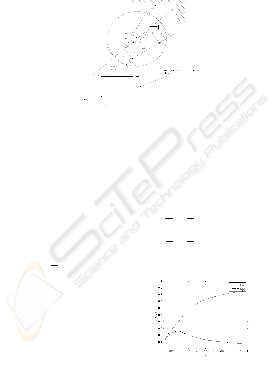
Figure 2: Angular contact ball bearing under thrust load.
heavily loaded rolling element, the approach of the
rings is,
ψαδαδδ
ψ
coscossin
ra
+=
(21)
At Ψ=0 maximum deflection occurs and is given
by
α
δ
α
δ
δ
cossin
max ra
+
=
(22)
Combining Equation (21) and (22) yields
)]cos1(
2
1
1[
max
ψ
ε
δδ
ψ
−−=
a
(23)
In which
)
tan
1(
2
1
r
a
δ
αδ
ε
+=
(24)
It should also be apparent that
5.1
max
)]cos1(
2
1
1[ ψ
ε
ψ
−−=
a
QQ
(25)
For static equilibrium to exist, the summation of
rolling element forces in each direction must equal
the applied load in that direction.
⎪
⎪
⎪
⎩
⎪
⎪
⎪
⎨
⎧
=
=
∑
∑
=
−=
=
−=
ψψ
ψψ
ψ
ψψ
ψψ
ψ
α
ψα
1
1
sin
coscos
QF
QF
r
r
(26)
In which Ψ
1
is the limiting angle defined as
follow,
)
tan
(cos
1
1
r
a
δ
αδ
ψ
−=
−
(27)
Using the integral form of J
r
(ε) and J
a
(ε)
introduced by Sjoväll, Equation (26) may be written
in equations system form.
⎪
⎭
⎪
⎬
⎫
⎪
⎩
⎪
⎨
⎧
+=
⎪
⎭
⎪
⎬
⎫
⎪
⎩
⎪
⎨
⎧
=
⎪
⎭
⎪
⎬
⎫
⎪
⎩
⎪
⎨
⎧
αε
αε
αδαδ
αε
αε
sin)(
cos)(
)cossin(
sin)(
cos)(
5.1
max
a
r
ra
a
r
a
r
J
J
ZK
J
J
ZQ
F
F
(28)
where J
r
(ε) and J
a
(ε) are defined as follows,
⎪
⎪
⎪
⎩
⎪
⎪
⎪
⎨
⎧
−−=
−−=
∫
∫
−
−
ψψ
επ
ε
ψψψ
επ
ε
ψ
ψ
ψ
ψ
dJ
dJ
a
r
5.1
5.1
1
1
1
1
)]cos1(
2
1
1[
2
1
)(
cos)]cos1(
2
1
1[
2
1
)(
(29)
The values of the integrals of Equation (28) can
be get using Simpson Integral Method, Fig.3 gives
the values of J
r
(ε) and J
a
(ε).
Figure 3: J
r
(ε) and J
a
(ε) vs. ε for angular contact ball
bearing.
ICINCO 2009 - 6th International Conference on Informatics in Control, Automation and Robotics
184

Figure 5: interface of calculation software for thermal contact resistance.
The nonlinear equations system has to be solved
by iteration, so the Newton-Raphson method can be
applied. When the axial deflection δ
a
and the thrust
deflection δ
r
is determined, the contact force on each
ball can be calculated by
5.1
5.1
)coscossin( ψδδδ
ψψ
aaKKQ
ra
+==
(30)
3.3 Contact Force Under Radial Load
Considering the structure of angular contact balling
bearing, when subjected to purely radial load F
r
, the
normal force Q
i
of the rolling element can be
decomposed into radial load component Q
ir
and axial
load component Q
ia
(as shown in Figure 4). The sum
of every axial load component was called derivative
axial force S, which can be calculated as follows:
α tan25.1
r
FS =
(31)
Figure 4: Derivative axial force.
To summarize, when rolling bearing is subjected
to purely radial load, an additional derivative axial
force is brought out. In this situation, the bearing can
be treated as being subjected to simultaneously to a
radial load and a centric thrust load.
4 CALCULATION SOFTWARE
AND AN EXAMPLE
4.1 Calculation Software
A calculation software has been made using the
MATLAB/GUI, whose interface is shown in Fig. 5
below.
The calculation procedure of thermal contact
resistance of ball bearing is as follows:
1) Input following parameters of the ball
bearing: ball diameter, ball number, radii of inner
and outer ring, ratio of inner and outer groove,
and the material properties, such as the modulus
of elasticity, Poisson's ratio and the thermal
conductivity.
2) Calculate the initial contact angle and the
load-deflection coefficient of the bearing, which
are useful in the calculation.
3) Define the loads of the bearing, and then
the load form is analysed.
a) If the radial load F
r
=0, a supposed axial
deflection value is needed.
b) If both the axial and radial loads are
positive, supposed axial and radial
deflection values must be input for the
THEORETICAL CALCULATION OF THERMAL CONTACT RESISTANCE OF BALL BEARING UNDER
DIFFERENT LOADS
185

calculation.
4) The axial/radial deflection value and the
final contact angle are calculated.
5) Finally, the normal load and thermal
contact resistance of each ball are obtained.
6) The overall thermal contact resistance of
the bearing can be get by connecting the thermal
resistance of each ball in parallel.
Take the following bearing as an example: the
bearing has 7 spherical balls, and all elements are
made from steel 440C; the diameter of the balls, 2r
b
,
is 9.525
mm ; the groove radii r
i
’ and r
o
’ are
1.03937r
b
, and the race radii r
i
and r
o
are 3.06037r
b
and 5.06562r
b
, respectively; the inner and outer
bearing diameters are 22mm and 56mm.
4.2 Contact Force Under Centric
Thrust Load
In this case, the bearing is subjected to varied thrust
load (F
a
) ranging from 20 to 200 N with a span of 10
N. The calculated thermal contact resistances are
shown in Figure 6.
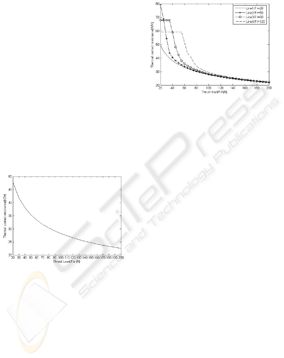
Figure 6: Thermal contact resistance under thrust load.
From Figure 6, we can see with the thrust load
increasing, the thermal contact resistance decreases.
That is because when the thrust load increases, the
normal load of each ball increases, then the contact
area extends.
4.3 Contact Force Under Combined
Radial and Thrust Load
In this case, the bearing is subjected simultaneously
to radial load of 20, 50, 80, 120 N, and varied thrust
load ranging from 20 to 200 N with a span of 5 N.
The calculated thermal contact resistances are shown
in Figure 7.
Figure 7: Thermal contact resistance under combined
thrust and radial load.
From Figure 7, we can see Line1 represents
much the same way as the line in Fig.4; While for
Line2, when the thrust load FA increases from 20 to
40 N, the thermal contact resistance changes rapidly.
That’s because the number of balls subjected to
normal load Q
i
changes from 1 to 4; For Line3,
when the thrust load FA changes from 20 to S
(derivative axial force, for F
r
=80N, S=38.5N),
because FA is smaller than S, the thrust load of the
bearing F
a
keeps F
a
=S, and the thermal contact
resistance stays at 67.76 W/K, with only 1 ball
subjected to normal load Q
i
. The following part of
Line3 represents the same way as Line2; Line4 is
like Line3.
In another way, for the thrust load FA=100N, the
contact resistance of each line is 27.80, 28.00, 28.41,
and 29.54, respectively. For combined thrust load
FA=100N and F
r
=20N, the contact resistance of
each ball (as shown in Fig.6) is 185.19, 188.53,
196.74 and 204.17, respectively; for FA=100N and
F
r
=50N, that is 173.85, 181.04, 201.08 and 223.07;
for FA=100N and F
r
=80N, that becomes 164.55,
174.68, 206.62 and 250.58; and for FA=100N and
F
r
=120N, that is 173.85, 181.04, 201.08 and 223.07,
respectively.
As mentioned above, the total contact resistance
is calculated by connecting that of every ball in
parallel. Since the load distribution of Line1 is much
more uniform than the others, the total contact
resistance of Line1 is smaller.
5 EXPERIMENTAL RESULTS
AND COMPARISON
A test program was conducted in order to verify the
prediction method of the thermal contact resistance.
ICINCO 2009 - 6th International Conference on Informatics in Control, Automation and Robotics
186

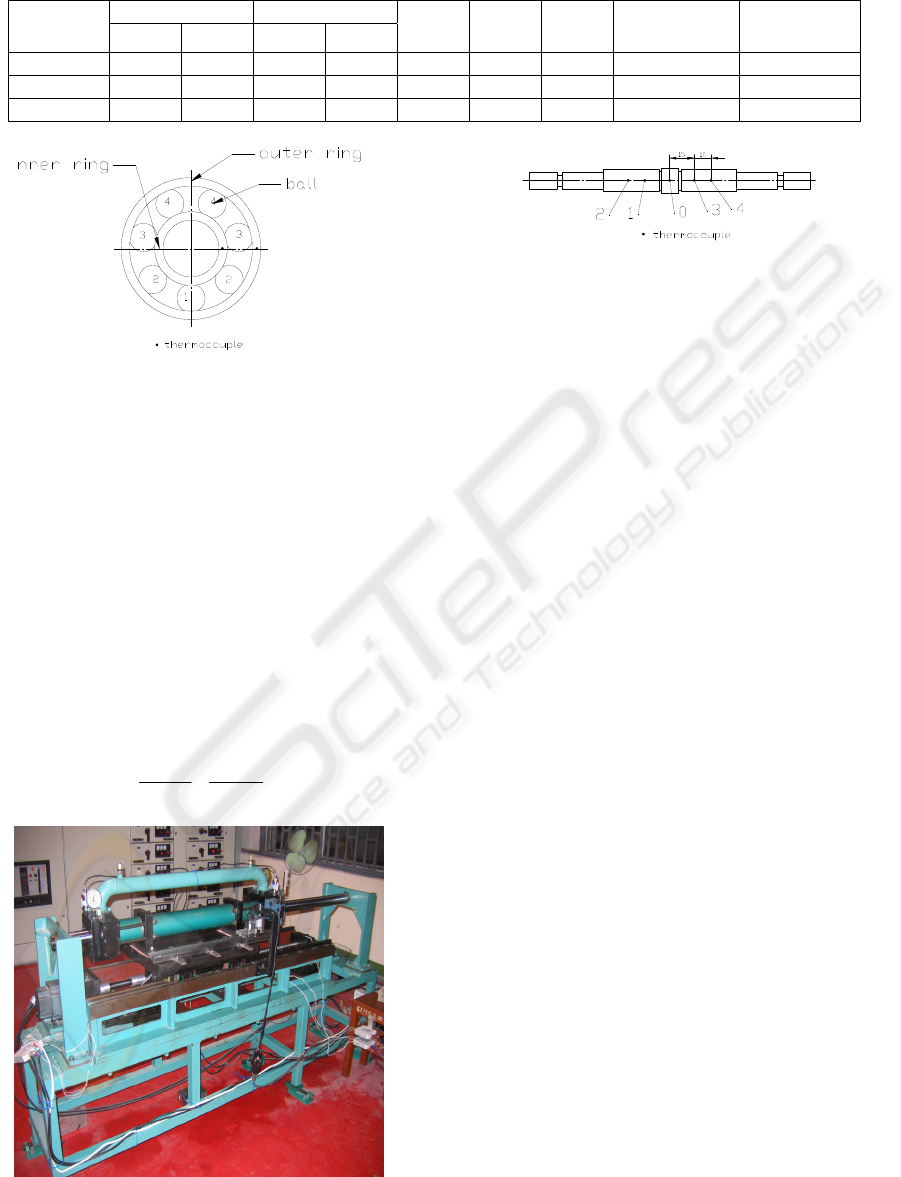
Table 1: Experimental results and predictions.
Test
Case no.
Load, N Temperature, K
Q, W
io
R
K/W
s
R
K/W
Measured, R
K/W
Predicted, R
K/W
Thrust Radial inner outer
1 39.2 0 298.2 334.8 0.88 41.59 2.2 39.39 38.24
2 0 98.1 300.3 336.8 0.54 67.3 2.2 65.1 63.30
3 39.2 39.2 300.3 329.1 0.68 42.60 2.2 40.40 39.44

Figure 8: Ball positions and temperature .measurement
points (Supposing the balls locate symmetrically).
The experimental apparatus is shown in Figure 9,
using thermocouples as sensors. The dimensions and
material properties of the bearing matched those
described previously. The thrust and radial load was
imposed by adjusting the pressure of the hydraulic
devices. Figure 8 and 10 show the temperature
measurement points on the bearing and the shaft.
The test parameters were shown in Table. The
temperatures shown in Table were obtained under
steady-state conditions when temperature changed
less than ±0.2
℃.
In the experiment, the bearing was considered as
the heat source. The conductive heat flow through
the shaft Q was calculated by,
)(
34
43
12
21
l
TT
l
TT
SkQ
s
−
+
−
=
(32)
Figure 9: High-speed experimental bench for thermal
contact resistance measurement.
Figure 10: Temperature measurement points on shaft.
Where T
i
, T
o
and R
s
denoted the measured
temperatures of the inner and outer rings, and the
conductive resistance for the solid existing between
the measurement points.
A comparison of the test result and the prediction
values is given in Table 1, and the agreement
between both results is excellent. Therefore, we can
say that the calculation method is applicable to the
prediction of contact resistance between the
elements of a angular contact ball bearing sustaining
thrust, radial and combined loads.
6 CONCLUSIONS
A calculation method based on precisely determined
contact forces has been presented to predict the
thermal contact resistance between the balls and the
inner and outer rings of a space-use dry bearing. The
study assumed that a stationary ball bearing
sustained axial, radial, or combined loads under a
steady-state temperature condition. While the
thermal analysis method is the same as that
employed to determine constriction resistance, the
assumptions commonly utilized in the constriction
problem have been numerically confirmed to be
applicable to the prediction of the contact resistance
between the bearing elements. Also, the calculation
of the contact resistance has indicated that the
careful consideration of changes in the contact angle
is important to determine the contact force and area
due to the axial loads.
For the load types dealt with, limited test data
were used to verify the proposed method because it
was not easy to get the same temperature
distribution across the bearing when the magnitude
of load was changed, and the total number of
operations had to be restricted to avoid changing the
surface condition. However, it can be said that the
THEORETICAL CALCULATION OF THERMAL CONTACT RESISTANCE OF BALL BEARING UNDER
DIFFERENT LOADS
187

excellent agreement between the test results and the
predictions has confirmed the applicability of the
proposed calculation method.
ACKNOWLEDGEMENTS
The work is supported by the National Natural
Science Foundation of China (No. 50675076), the
National Key Basic Research Special Found of
China (No.2005CB724100) and National Natural
Science Foundation of China (No. 50575087).
REFERENCES
Yovanovich, M. M., 1975. Thermal Constriction
Resistance of Contacts on a Half-Space: Integral
Formulation, AIAA Paper 75-708.
Clausing, A. M., Chao, B. T., 1965. Thermal Contact
Resistance in Vacuum Environment, Transactions of
the American Society of Mechanical Engineers, Ser.
C., Vol. 87: 243-251.
Madhusudana, C. V., Fletcher, L. S., 1986. Contact Heat
Transfer—the Last Decade, AIAA Journal, Vol. 24,
No. 3:510-523.
Yovanovich, M. M., 1986. Recent Development in
Thermal Contact, Gap and Joint Conductance Theories
and Experiment, Proceedings of the 8th International
Heat Transfer Conference (San Francisco, CA): 35-
45.
Yovanovich, M. M., 1986. Thermal Contact Resistance
Across Elastically Deformed Spheres, Journal of
Spacecraft and Rockets, Vol.4, No. 1: 119-12.
Yovanovich, M. M., 1986. Thermal Constriction
Resistance Between Contacting Metallic Paraboloids:
Application to Instrument Bearings, AIAA Paper 70-
857.
Love, A. E. H., 1944. A Treatise on the Mathematical
Theory of Elasticity, Dover, New York, 4
th
edition.
Cooper, D. H., 1969. Hertzian Contact-Stress Deformation
Coefficients, Journal of Applied Mechanics, Vol. 36:
296-303.
Harris, T.A., 2001. Rolling Bearing Analysis, John Wiley
& Sons, Inc., New York, 5
th
edition
ICINCO 2009 - 6th International Conference on Informatics in Control, Automation and Robotics
188