
A NEW APPROACH OF THE NEURAL PREDICTIVE CONTROL
APPLIED IN A THERMOELECTRIC MODULE
Adhemar de Barros Fontes, Pablo Amorim and M´arcio Ribeiro da Silva Garcia
Departamento de Engenharia El´etrica, Universidade Federal da Bahia, Rua Aristides Novis 2 Federac˜ao, Salvador, Brazil
Keywords:
Neural Control, Neural Networks, Nonlinear systems, Predictive Control.
Abstract:
This article presents an efficient solution for predictive control based on neural networks with feedfoward
multilayer, as a model for a thermoelectric module. It is shown the capability of a neural network to learn
the entire nonlinear dynamics and the advantage of using these nonlinear models for the calculation of the
predicted variables. It is also suggested a new control law capable of minimize the cost function using the
Newton-Raphson and the descendent gradient optimization rules. For this application it is shown that a sig-
nificant reduction in the number of iterations and application in real-time systems when compared to other
optimization techniques.
1 INTRODUCTION
The recursive neural networks have shown to be a
very important tool in several control applications in
nonlinear dynamic systems. This article has the ob-
jective os presenting a development and its results ob-
tained from a prediction-based algorithm through a
recursive neural network applied in a thermoelectric
chamber with nonlinear dynamics.
The Generalized Preditive Controller (GPC) was
introduced by (Clarke, 1994) and is being used for
control of industrial process with profitasble perfor-
mance in the control of non-minimum phase plants,
unstable plants or plants with unknown dead time
(Clarke, 1994). The GPC uses initially a linear predic-
tion model. If a nonlinear model is used then it is also
necessary to make use of a nonlinear algorithm. Ex-
pressive results are obtained regarding efficiency and
computational performance. The prediction feature of
the GPC when using a neural model, with the capa-
bility of learning the entire dynamic of the plant, it is
more efficient than the standard nonlinear modelling
techniques. It is well known that the plant model is di-
rectly related to the accuracy of the prediction (Fontes
et al., 2008). The most used techniques to modelling
nonlinear plants, as the linearization around the op-
erating points (Lee and Ricker, 1994; Li and Biegler,
1988) or approximated models, do not guarantee the
required accuracy when compared to the neural mod-
els.
The control signal update rule in the present work
is based on the first and second derivatives of the cost
function. A new hybrid control law is proposed based
on the Newton-Raphson rules and the decrecent gra-
dient. The computational cost related to the computa-
tion of the control signal is associated to the Hessian.
However, the reduced number of iterations guarantee
an excelent performance of the algorithm when it is
applied in real-time control systems.
For simulation and real trials of the proposed con-
trol technique a Peltier cell was mounted in a set
named the thermoeletric chamber. The results ob-
tained caracterize a suitable solution for the proposed
system, as well as the potential of this tool in the mod-
elling and control of nonlinear systems, whenever it
is real-time or not. In the section 2, the structure of
a recursive neural network is presented as well as the
equations that describe it. In the section 3, the neces-
sary equations for the determination of the proposed
control law. The section 4 presents the description
and modelling of the system as well as the results ob-
tained in the trials.
2 NEURAL NETWORK
ARCHITETURE
The model of a plant used in a neural generalized pre-
dictive controller (NGPC) is a neural network and it
is important to evaluate the architeture of the network
to be used. It is known that a recursive neural net-
189
de Barros Fontes A., Amorim P. and Ribeiro da Silva Garcia M. (2009).
A NEW APPROACH OF THE NEURAL PREDICTIVE CONTROL APPLIED IN A THERMOELECTRIC MODULE.
In Proceedings of the 6th International Conference on Informatics in Control, Automation and Robotics - Intelligent Control Systems and Optimization,
pages 189-194
DOI: 10.5220/0002193001890194
Copyright
c
SciTePress
work with three layers, one of them hidden, is capa-
ble of representing any linear or nonlinear function.
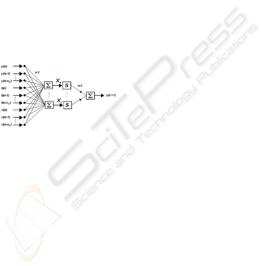
The Figure 1 describes a multilayer feedforward neu-
ral network with all its structure of delayed inputs and
outputs signals. In (Hao et al., 1993), it was presented
in details the mathematical representation of nonlin-
ear plants and the respective considerations in order
to determine the order of the neural model in terms of
the regressors of the inputs, disturbances and outputs,
namely, u(n), t(n) and y(n). For each perceptron of
the hidden layer there is an activation function. The
neural network is described by the following equa-
tion:
y(n+ 1) = f(y(n), y(n− 1), . . . , y(n − n
y
), t(n), . . . ,
t(n− n
t
), u(n), . . . , u(n− n
u
)),
(1)
or, in a detalied view,
Figure 1: The recursive neural model structure.
y(n+ 1) =
N
∑
i=1
w
2
(1, i)S(X
i
), (2)
with,
X
i
=
∑
n
y
j=1
w
1
(i, j)y(n− j)+
∑
n
t
j=0
w
1
(i, n
y
+ 1+ j)t(n− j)+
∑
n
u
j=0
w
1
(i, n
y
+ n
t
+ 2+ j)u(n − j),
(3)
where:
• y(n+ 1) is the output of the neural network;
• S(.) is the output function of the i − th nodes of
the hidden layer;
• N is the number of nodes in the hidden layer;
• n
y
is the number of inputs nodes associated to y(.);
• n
t
is the number of inputs nodes associated to t(.);
• n
u
is the number of inputs nodes associated to
u(.);
• w
1
(i, j) represent the weights associated of the j−
th input to the node j;
• w
2
(1, i) represent the weights associated of the i−
th hidden node to the output node;
• y(.) represents the output past values;
• t(.) represents the ambient temperature past val-
ues;
• u(.) represents the input past values.
3 OPTIMIZATION
For the presented application it is necessary the use
of a cost function with finite prediction horizon. The
NGPC algorithm must satisfy the following optimiza-
tion problem:
∆u(k) = min
∆u
n
J =
∑
N
2
i=N
1
||ref(n+ i) − ˆy(n+ i)||
2
+
λ
∑
N
u
i=1
||∆u(n+ i)||
2
o
,
(4)
where:
• N
1
is the minimum prediction horizon;
• N
2
is the maximum prediction horizon;
• N
u
is the control horizon;
• ref(n+ i) is the reference signal;
• ˆy is the output signal predicted by the neural
model;
• λ is the weight at the control signal;
• ∆u(n+ i) is the variation of the control signal de-
fined as u(n+ i) − u(n+ i− 1).
For the cost defined in (4) there are four tuning
parameters: N
1
, N
2
, N
u
and λ. As the dead time is
much smaller than the sampling time, it is fair to ad-
mit N
1
= 1 and, as a consequence, N
2
= N
u
. It may
be verified also that, while the cost is minimized, the
resulting control signal allows the plant to track the
reference signal.
As mentioned before, the proposed control law
presents an update algorithm based on the rules of
Newton-Raphson and the decrecent gradient. The use
of two methods allows the adding of the weight α,
according to (5). This way, the control law contem-
plates one more degree of freedom and as a conse-
quence a gain in the dynamics of the controller. The
control law proposed for the update of the control sig-
nal U(k+ 1) is given by,
ICINCO 2009 - 6th International Conference on Informatics in Control, Automation and Robotics
190
U(k+ 1) = U(k) − α
∂J
∂U
− (
∂
2
J
∂U
2
)
−1
∂J
∂U
(5)
It is easily observed that there’s an addition of a
new degree of freedom α, besides the one defined in
(4). The optimal value of J in terms of U is obtained
after each iteration of the optimization algorithm. In
the iterative process, for each value of J the future in-
puts vector U(k) is also calculated, with the Jacobian
and Hessian matrices defined as:
∂J
∂U
=
∂J
∂u(n+1)
∂J
∂u(n+2)
···
∂J
∂u(n+N
u
)
, n = 1, . . . , N
u
(6)
∂
2
J
∂U
2
=
∂
2
J
∂u(n+1)
2
. . .
∂
2
J
∂u(n+1)∂u(n+N
u
)
···
.
.
.
···
∂
2
J
∂u(n+N
u
)∂u(n+1)
. . .
∂
2
J
∂u(n+N
u
)
2
,
(7)
and the predicted output is given by:
ˆy(n+ k) =
N
∑
i=1
w
2
(1, i)S(X
i
). (8)
The iterations are interrupted when the percentage
of the variation U(k) is smaller than a given ε. For
each iteration k the elements of the Jacobian and the
Hessian are calculated for the given control law.
It is necessary that efficient routines are elaborated
for the calculation of the gradient, used in the mini-
mization of the cost, when the iterations of the opti-
mization algorithm are used in real-time.
4 TRIALS
4.1 System Description
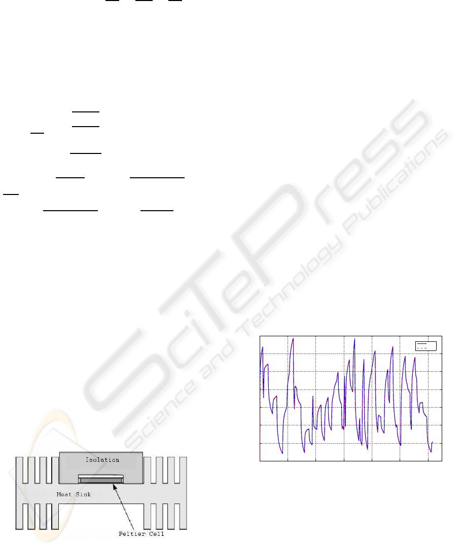
Figure 2: Thermoelectric module.
A Peltier cell, also know as thermoelectric module
(TEM),is a component composed of several semi-
conductors plates placed side-by-side and electrically
isolated from the external environment by a ceramic
coat. Through two terminals connected to the cell
a electric current circles, causing the heat to pump
between its faces. This phenomenon is know as the
Peltier efect and it is the opposite of the Seebeck
efect, which caracterizes the thermocouples. The heat
pumpingdirection depends on the direction of the cur-
rent flow, which allows the Peltier cells to be used as
actuators in cooling systems as much as in heating
systems.
The TEM is widely used in temperature control in
specific applications (Fontes et al., 2008). In some
of them a physical model is used, (Fontana, 2001;
Almeida, 2003). These applications vary from cool-
ing modules, medical instruments composition and
small refrigerators, etc (Mel, 1999).
A thermoelectric module is composed of a ther-
mic chamber, where the Peltier cell is associated to a
heat sink. The Figure 2 presents an illustration of the
set used in the experiments of heat pumping. The pro-
cess variable is the upper face temperature, controlled
by the manipulation of the applied current. The infor-
mation of the ambient temperature is also informed to
the neural net as a load disturbance. Other works in-
volving the thermic chamber present a caracterization
of the module by nonlinear parametric models (So-
brinho et al., 2006; Lima, 2007; Almeida, 2004) and
bilinear state-space models (Garcia, 2008).
4.2 Neural Network Training
0 100 200 300 400 500 600
35
40
45
50
55
60
65
70
Temperature (
o
C)
Real
Model
Figure 3: Neural model plot versus system’s real data.
For the network trainning, the system response for
a Pseudo-random signal input (PRS) was obtained
along the entire operation range (30
o
C a 80
o
C). The
proposed architeture for the neural model contem-
plates 3 layers, with 3 regressors in the hidden layer
and one in the output layer, 3 exogen regressors and
the Hyperbolic Tangent as the activation function;
During the training phase the weights were ad-
justed iteratively, as proposed in (Hagan and Men-
A NEW APPROACH OF THE NEURAL PREDICTIVE CONTROL APPLIED IN A THERMOELECTRIC MODULE
191
haj, 1994). For the feedforward architeture proposed,
the performance was measured in acordance with the
minimization of the squared error criterion between
the network and the system’s real outputs for the
same input signal. Several training algorithms were
used, as the resilient backpropagation, the Fletcher-
Reeves rule with backpropagation of the conjugated
gradient, the Polak-Ribiere rules, the decrescent gra-
dient, among others. The algorithm of Levenberg-
Marquardt presented the best overall results and it was
used for the system modeling. The Figure 3 presents
the output of the neural model compared to the real
system’s output.
For validation, another PRS was generated and ap-
plied to the system and its response was compared to
the model response. The mean squared error between
the system (y
r
) and the model ( ˆy
m
) outputs for the N
points, defined as
E
mq
(%) =
q
∑
N
i=1
(y
r
− ˆy
m
)
2
N
∗ 100, (9)
was 1, 148%
The closed-loop system was implemented accord-
ing to the well-known receiding horizon principle
((Propoi, 1963; Camacho and Bordons, 2004; Za-
marreo and Vega, 1999)). It is fair to say that the good
computationalperformanceof the proposedcontroller
is based on the choice of the algorithm defined in
the optimization block. The choice of the controller
parameters can be done by several criteria: Num-
ber of iterations for the resolution of the control sig-
nal, computational cost and accuracy of the solution.
It is necessary though, to develop fast optimization
algorithms. In this works a solution is presented,
which applies the Newton-Raphson method added by
the decrecent gradient which can be implemented as
optimization technique in highly nonlinear real-time
applications. A computational analysis showed that
there was no significant increase in the computational
cost associated with the optimization of the control
signal with the increment of the decendent gradient
method. The terms of the decrecent gradient to be
calculated are the same as the onse of the Newton-
Raphson’s method.
4.3 Results
The trials were performed for three distinct cases: The
algorithm 01 represents the system proposed in this
article with parameters λ = 2000 and α = 0.00008.
The algorithm 02 refers to the same algorithm with
a more agressive tuning (α = 0.0000955). The algo-
rithm 03 refers to an existing algorithm, without the
addition of the term related to the decrecent gradient,
with λ = 2000. The prediction horizon is Ny = 10.
The small values of α are due to the system’s large
static gain, but the variation of these parameters be-
tween the algorithms 1 and 2 is 20%.
0 1000 2000 3000 4000 5000 6000 7000
−3
−2
−1
0
1
2
3
Ambient temperature
Reference
Controled Temperature
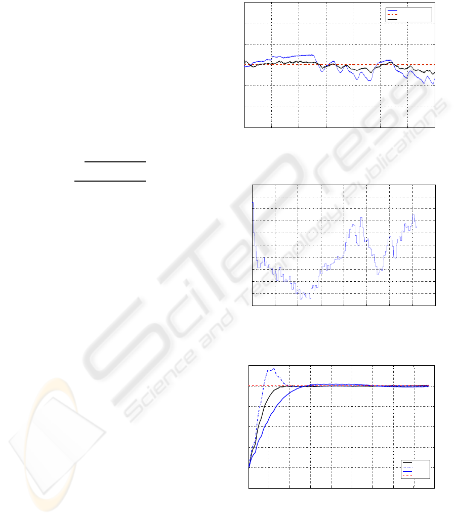
Figure 4: System response to load disturbances.
0 1000 2000 3000 4000 5000 6000 7000 8000
0.488
0.49
0.492
0.494
0.496
0.498
0.5
0.502
0.504
0.506
0.508
Time (s)
Control Signal (V)
Control Signal With The NGPC − Regulator Case
Figure 5: Control signal for the regulator case.
0 200 400 600 800 1000 1200 1400 1600 1800
30
35
40
45
50
55
60
Time (s)
Controlled Temperature (ºC)
System Response With The NGPC Controller
Algorithm 1
Algorithm 2
Algorithm 3
Reference
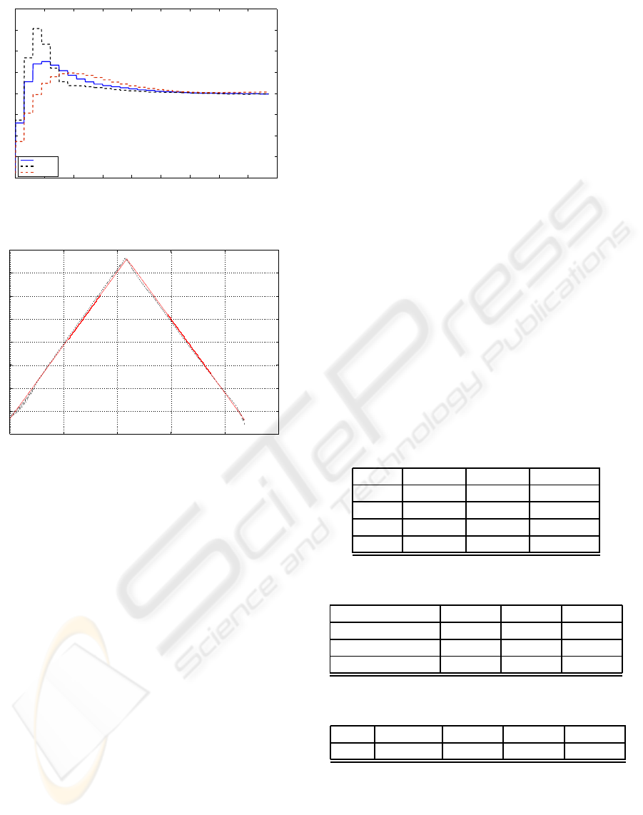
Figure 6: System response for a step in the reference.
The Figure 4 shows the system response to a dis-
turbance caused by the variation of the ambient tem-
perature. It is easy to observe that the controller is ca-
pable of rejecting the distubance, keeping the system
ICINCO 2009 - 6th International Conference on Informatics in Control, Automation and Robotics
192
0 200 400 600 800 1000 1200 1400 1600 1800
0.1
0.2
0.3
0.4
0.5
0.6
0.7
0.8
0.9
Time (s)
Control Signal (V)
Control Signal With The NGPC − Servo Case
Algorithm 1
Algorithm 2
Algorithm 3
Figure 7: Control signals for the servo case.
0 0.5 1 1.5 2 2.5
x 10
4
30
35
40
45
50
55
60
65
70
Time (s)
System’s Response − Ramp Reference
Figure 8: System response for a ramp reference.
output inside the desireble range, presenting a very
small offset of 0.3
o
C, inside the accuracy range of
the sensors, for an ambient temperature variation of
1.5
o
C. The output signal of the controller for this case
is shown in the Figure 5.
The system response for a deviation of 20
o
C in
the setpoint for the three controllers implemented is
shown in the Figure 6, in which the dashed line rep-
resents the system output for the algorithm 02, while
the black and blue lines represent the algorithms 01
and 03 respectivaly. The control signal for the three
algorithms are expressed in the Figure 7.
For better evaluation of the performance of the
controllers, the indices presented in (Goodhart et al.,
1994) were used, which are the mean and variance of
the controller outputs ( ¯u and σ
u
, respectivaly), the In-
tegral of the Absolute Error (IAE), which penalizes
the error between the reference and the system vari-
able and the Integral with Time of the Absolute Error
(ITAE), which penalizes the absolute error through-
out the time line. The calculated indices are shown in
the Table 1 and the time parameters of the closed-loop
system is presented in the Table 2. It is easy to see that
the algorithm proposed in the present work presents
a better performance in relation to the tracking error
and a smaller mean control effort(¯u). The settling time
is also smaller. The rise time for the second algorithm
is smaller, but it also presents a large overshoot which
may not be viable in real applications. For the regula-
tory trial, the results obtained were E
qm
= 0.0755%,
IAE = 0.104, ITAE = 145.108.
The third and last trial was the analyzis of the
system response for a ramp reference. The control
law does not contemplate a second integral action,
necessary for the ramp tracking. Still, the algorithm
provided good results when compared to other tech-
niques. In this work, the proposed methodology was
compared to three other results obtained for differ-
ent controllers for the same case: The algorithm B
is a single model based GPC presented in (Lima,
2007). The algorithms C and D are described in (San-
tana, 2008) in a multi-model environment, with the
controllers based on gain margin and phase margin
metrics, respectively. The algorithm A is the one
proposed in this work, with Ny = 2, λ = 3000 and
α = 0.000095. The ramp started in the temperature of
33.5
o
C covering all modeled range with variation of
0.1915
o
C at each 60 seconds, which corresponds to
one sampling time. The overall results are shown in
Table 3
Table 1: Performance indices for the controllers.
Alg. 01 Alg. 02 Alg. 03
¯u 0.5295 0.5332 0.5196
σ
u
0.0031 0.0063 000038
IAE 0.6728 0.6226 1.1550
ITAE 77,1668 81,7647 244,9661
Table 2: Time indices for the controllers.
Alg. 01 Alg. 02 Alg. 03
Rise Time 200s 118s 358s
Settling Time 296s 354s 972s
Max. Overshoot 0% 21.66% 2.21%
Table 3: Mean squared error for a ramp reference.
Alg. A Alg. B Alg. C Alg. D
Eqm 0.3191% 2.214% 1.482% 1.418%
The neural networks is capable of capturing the
entire dynamic of the system. Performance indices
based on the number of iterations and the computa-
tional effort when only the jacobian is used was pre-
sented in (Soloway and Halcy, 1996). It is fair to af-
firm that the reduced number of iterations performed
by the NGPC algorithm ranges from 6 to 12 times
A NEW APPROACH OF THE NEURAL PREDICTIVE CONTROL APPLIED IN A THERMOELECTRIC MODULE
193

faster, even with the calculation of the Hessian requir-
ing a high computational effort.
5 CONCLUSIONS
In this work a new approach of the Neural GPC was
presented which complies a little modification in the
control law, given by the adding of one more degree
of freedom associated to the decrecent gradient. This
modification caused a significant improvement in the
control effort and in the general system’s closed-loop
response without significant increase of the compu-
tational effort. Furthermore, the algorithm becomes
much more flexible when compared to other one-
degree of freedom based strategies.
The trials were executed in a real-time nonlin-
ear physical system with complex dynamics, with
non-minimum phase states and highly nonlinear static
gains along the diferente operation ranges. The neu-
ral model was able to represent with very good accu-
racy the system dynamics, which shows the efficiency
of the neural networks when applied in the nonlinear
system identification. The system was implemented
to prove in practice the superior performance of the
proposed technique. The same algorithm may be ap-
plied in the control of important industrial process,
as in multivariable control, level, concentration and
temperature. The developed algorithm may estim-
ulate new applications involving the ideas presented
in this work. The low computational cost allows the
practical implementation of the proposed algorithm in
real-time existing embedded systems.
REFERENCES
(1999). Theromeletric coolers and accessories. Melcor
Corporation, first edition.
Almeida, L. A. L. (2003). Modelo de Histerese para
Transic˜ao Semicondutor-Metal em Filmes Finos de
VO2. PhD thesis, Universidade Federal de Campina
Grande.
Almeida, L. A. L. (2004). Modelo dinmico n˜ao-linear para
m´odulo termoel´etrico. In XV Congresso Brasileiro de
Automtica.
Camacho, E. F. and Bordons, C. (2004). Model predictive
control. Springer-Verlag Limited.
Clarke, D. W. (1994). Advanced in model-based predictive
control. Oxford Univesity Press.
Fontana, M. (2001). Caracterizac˜ao e modelagem das pro-
priedades ´opticas de sensores de di´oxido de van´adio.
Master’s thesis, Universidade Federal de Campina
Grande.
Fontes, A. B., Dorea, C. E. T., and Garcia, M. R. S. (2008).
An iterative algorithm forconstrained mpc with stabil-
ity of bilinear systems. In 16th Mediterranean Confer-
ence on Control and Automation, pages 1526–1531.
Garcia, M. R. S. (2008). Controle preditivo por realimen-
tac˜ao de estado de sistemas bilineares sob restric˜oes
aplicado a um m´odulo termoel´etrico. Master’s thesis,
Universidade Federal da Bahia.
Goodhart, S. G., Burnham, K. J., and James, D. J. G.
(1994). Bilinear self-tuning control of a high temper-
ature heat treatment plant. IEE Proc.-Control Theory
Appl., 141(1):12–18.
Hagan, M. T. and Menhaj, M. (1994). Trainning feedfor-
ward networks with the marquadt algorithm. IEEE
Transactions on Neural Networks, 5(6):989–993.
Hao, J., Tan, S., and Vandewalle, J. (1993). One step ahead
predictive control of nonlinear systems by neural net-
works. In Proceedings of 1993 International Joint
Conference on Neural Networks.
Lee, J. H. and Ricker, N. L. (1994). Extended kalman filter
based nonlinear model predictive control. Ind. Eng.
Chem. Res., 33(6):1530–1541.
Li, W. C. and Biegler, L. T. (1988). Process control strate-
gies for constrained nonlinear systems. Ind. Eng.
Chem. Res., (27):1421–1433.
Lima, J. S. (2007). T´ecnicas de controle preditivo bilinear
aplicado a um m´odulo termoel´etrico. Master’s thesis,
Universidade Federal da Bahia.
Propoi, A. I. (1963). Use of lp methods for synthesiz-
ing sampled-data automatic systems. Automn Remote
Control, 24.
Santana, M. J. C. (2008). Controle preditivo multimod-
elo aplicado a um m´odulo termoel´etrico: Uma nova
m´etrica. Master’s thesis, Universidade Federal da
Bahia.
Sobrinho, M. O. S. L., Lima, J. S., Souza, V. O. S. T.,
Fontes, A. B., and Almeida, L. A. L. (2006). Car-
acterizac˜ao de um m´odulo termoel´etrico por modelo
param´etrico bilinear. Congresso Brasileiro de Au-
tomtica.
Soloway, D. and Halcy, P. J. (1996). Neural generalized pre-
dictive control, a newton-raphason implementation. In
Symposium on Intelligent Control.
Zamarreo, J. M. and Vega, P. (1999). Neural predictive con-
trol. application to a highly non-linear system. En-
gineering Applications of Artificial IntelligenceJapan,
(12):149–158.
ICINCO 2009 - 6th International Conference on Informatics in Control, Automation and Robotics
194
