MODELING, SIMULATION AND FEEDBACK LINEARIZATION
CONTROL OF NONLINEAR SURFACE VESSELS
Mehmet Haklidir, Deniz Aldogan, Isa Tasdelen and Semuel Franko
TUBITAK Marmara Research Centre, Information Technologies Institute, 41470, Gebze-Kocaeli, Turkey
Keywords: Surface Vessels, Nonlinear Analysis and Control, Feedback Linearization.
Abstract: Realistic models and robust control are vital to reach a sufficient fidelity in military simulation projects
including surface vessels. In this study, a nonlinear model including sea-state modelling is obtained and
feedback linearization control is implemented in this model. To control the system, nonlinear analysis
techniques are used. The model is integrated into a commercial framework based CGF application within a
high-fidelity military training simulation.The simulation results are presented at the end of the study.
1 INTRODUCTION
The aim of this study is to observe the dynamic
behaviors of the surface vessels under the effect of
hydrodynamic force-moments and environmental
conditions such as waves, current, wind, season that
pertaining to the tactical environment.
The analysis and control of nonlinear motion
model of surface vessels are obtained by using
following techniques:
• Linearization by Taylor Series
• Phase Plane Analysis
o Course Keeping
o Zig Zag Maneuver
• Lyapunov Stability Theorem
• Feedback Linearization
Ship dynamics model and disturbance model are
introduced in Section 2; the phase plane analysis and
lyapunov stability therom in Section 3 and 4, the
proposed controller is discussed in Section 5;
simulation results are presented in Section 6.
2 THE SURFACE PLATFORM
MOTION MODULE
2.1 Coordinate System and Vector
Notation
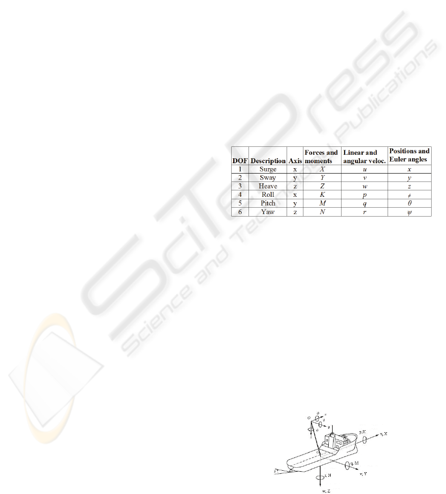
The motion of surface vessels has 6 degrees of
freedom. The description and notation of each
degree of freedom has been shown on Table 1.
Table 1: DoF Description and Notation.
SNAME’s (1950) notation is used in this study.
The first three parameters and time derivatives that
are shown on Table define the position and the
motion of the platform in x-, y-, z- axes. Last three
parameters define the orientation and rotary motion
of the platform. After analyzing 6 degrees of
freedom motion of surface vessel, it is observed that
2 axis systems are needed to perform the motion.
Therefore, North – East- Down (NED), is the local
geodetic coordinate system fixed to the Earth, and
Body Fixed, is fixed to the hull of ship, coordinate
frames are used. Motion axis system X
0
Y
0
Z
0
has
been fixed to the platform and called as Body Fixed
axes system. The point O, which is the origin of this
axes system, is always selected as the ship’s centre
of gravity. (Figure 1)
Figure 1: Coordinate System.
92
Haklidir M., Aldogan D., Tasdelen I. and Franko S. (2009).
MODELING, SIMULATION AND FEEDBACK LINEARIZATION CONTROL OF NONLINEAR SURFACE VESSELS.
In Proceedings of the 6th International Conference on Informatics in Control, Automation and Robotics - Signal Processing, Systems Modeling and
Control, pages 92-97
DOI: 10.5220/0002194300920097
Copyright
c
 SciTePress

2.2 Surface Platform Motion Equations
Fossen (1991), by inspiring Craig’s (1989) robot
model, contrary to classical representation, modeled
6 degrees of freedom motion of the surface vessel
vectorially.
()J=ηηυ

() () ()MC D+++=υυυυυg ητ

+g
0
+w
Above; M is the moment of inertia including
added mass, C(υ) is Coriolis matrix, D(υ) is
damping matrix, g(η) is gravitational force vector
and τ is the vector showing the force and moments
of the propulsion system that causes motion. This
representation will be used in this study.
2.2.1 Motion Equations
Representing the motion equations in the Cartesian
system of coordinates (body-fixed reference frame)
and defining x
G
, y
G
and z
G
as the position of the
ship’s CG, the well known motion equations of a
rigid body are giving by the following (Fossen,
1991):
Surge:
22
[()()()]
GGG
X
m u qw rv x q r y pq r z rp q=+−+ ++ −+ +

Sway:
22
[()()()]
GGG
Ymvrupwyr p zqrp xqpr=+−− ++ −+ +

Heave:
22
[()()()]
GGG
Z
m w pv qu z p q x rp q y rq p=+−− ++ −+ +

Roll :
()[( )( )]
XZy G G
K I p I I qr m y w pv qu z u ru pw=+− + +−−+−

Pitch:
()[( )( )]
yxZ G G
M
Iq I I rp mz u qw rv x w pv qu=+− + +−− +−

Yaw:
()[( )( )]
Zyx G G
N I r I I pq m x v ru pw y u qw rv=+− + +−− +−

2.2.2 Simplifying Assumptions
Simplifying assumptions used in this study are
following:
• The rotational velocity and acceleration about
the y-axis are zero (q, = 0).
• The translational velocity and acceleration in
the z direction are zero. (w, = 0).
• The vertical heave and pitch motions are
decoupled from the horizontal plane motions.
• The vertical centre of gravity, (VCG), is on the
centerline and symmetrical (yG=0)
2.2.3 Simplified Motion Equations
Applying simplifying assumptions to the general
motion equations, the following simplified equations
of motion are obtained
Surge:
2
[]
GG
X
mu rv x r z rp=−− +

(1)
Sway:
[]
GG
Ymvruzpxr
=
+− +

(2)
Roll:
()]
XG
K
Ipmz uru
=
−+

(3)
Yaw:
()
ZG
NIrmxvru
=
++

(4)
2.2.4 Force and Moments Acting on Surface
Vessel
Basically force and moments acting on surface
vessel can be divided to four as; hydrodynamics
force and moments, external (environmental) loads,
control surface forces (rudder, fin..) and propulsion
(propeller) forces. Force and moments can be
expressed according to axis system;
Surge: X = X
H
+ X
R
+ X
E
+ T
Sway: Y = Y
H
+ Y
R
+ Y
E
Roll: K = K
H
+ K
R
+ K
E
Yaw: N = N
H
+ N
R
+ N
E
Description of indices is; H, Hydrodynamic
force and moments originating from fluid-structure
interaction, R , forces that affects control surface are,
E, environmental external loads (Wave, current,
wind), T, propulsion force.
Hydrodynamic Forces and Moments
Integration of the water pressure along the wetted
area of the surface vessel causes hydrodynamic force
and moments within the platform. These force and
moments can be defined, with the velocity and
acceleration terms as a nonlinear axes system, by
using Abkowitz method.
Most important step on developing maneuver
model is expanding force and moment terms in
Taylor’s series. This way, nonlinear terms act as
independent variables and form a polynomial
equation. The function and its derivatives have to be
continuous and finite in the region of values of the
variables to use the Taylor's expansion. Certainty of
the model alters depending on where the expansion
is finished.
Force and moments, which were obtained by
expanding Taylor series until third power, are under
mentioned (Abkowitz, 1969; Sicuro, 2003)
2
()
hid u vr uu
X
Xu Xvr Xv=++


(5)
hid v r p
uv ur
ur
uu u v v v
vr rv
YYvYrYpYuvYur
YuuYuvYurYvv
Yvr Yrv
φφ
φ
φφ
φ
=++ + +
++++
++
 
 
(6)
MODELING, SIMULATION AND FEEDBACK LINEARIZATION CONTROL OF NONLINEAR SURFACE VESSELS
93

()
hid v p ur
uv vv
vr rv uv
uu
ur u p
pz
pp
KKvKpKuvKurKvv
Kvr Krv K uv
Kur KuuKup
KppKpK G
φ
φ
φ
φφφ
φ
φφ
φ
φφ φ
=+ + + +
++ +
+++
+++−Δ


(7)
Obtaining Hydrodynamic Derivatives
In order to obtain hydrodynamic derivatives three
basic methods can be used.
¾ By means of basin test using the realistic
model
¾ By using CFD (Computational Fluid
Dynamics) software
¾ By using empirical formulae
In this study third method was used.
Hydrodynamic derivatives have been used by the
empirical formulae of the source Inoue et al. (1981).
To have an opinion about validity and fidelity of the
empirical formulae, parameters of a merchant ship
that was chosen from literature was used. By using
these parameters and related formulae hydrodynamic
derivatives were calculated and compared with the
equivalent in the literature.(Table 2)
Table 2: Comparing the hydrodynamic derivatives
obtained from the model data and empirical formulae.
The Environmental Disturbances
The environmental disturbances acting on the
surface vessels can be grouped into two main
categories; the wave model, the current and wind
models.
The Wave Model
When real data regarding the complicated seas lacks,
idealized mathematical spectrum functions are
generally used for marine calculations. One of the
easiest and commonly used of these calculations is
the Pierson – Moskowitz spectrum where a wave
spectrum formula is provided for winds blowing
over an infinite area and at a constant speed for over
a sea of full state. In this study this spectrum is used
while a wave model is created.(Berteaux, 1976)
This spectrum is expressed as follows due to the
wave frequency and wind speed.
4
2
5
0.0081g g
S exp 0.74
V
ξ
⎡
⎤
⎛⎞
=−
⎢
⎥
⎜⎟
ω
ω
⎝⎠
⎢
⎥
⎣
⎦
(8)
where, ω : Wave Frequency [rad/sec], V: Wind
Speed (at 19,5 m above sea) [m/s]
The Current and Wind Models
Typically wind models only treat the force and
moments that are directly related to surge, sway and
yaw motions. In this study, the wind model is
obtained by using Isherwood Method.(Isherwood
1972)
Wind forces and moments acting on a surface
platform are usually defined in terms of relative
wind speed V
R
(knots) and relative angle γ
R
(deg).
The wind forces for surge and sway and the wind
moment for yaw as is shown.
2
1
()
2
wr X R w R T
X
CVA γρ =
(9)
2
1
()
2
wr Y R w R L
YC VA γρ =
(10)
2
1
()
2
wr N R w R L
NC VAL γρ =
(11)
where C
X
, C
Y
and C
N
are the force and moment
coefficients, ρw is the density of the air, AT and AL
are the transverse and lateral projected areas and L is
the overall length of the ship. (Isherwood, 1972).
The equations of current forces and moments are
similar with wind forces and moments.
2.3 Nonlinear Equations of Motion
When the simplified 4 degrees of freedom motion
model, which was obtained in previous section, was
associated with hydrodynamic forces and
environmental external loads a nonlinear maneuver
model can be obtained. To behave like independent
variables and become coefficients of a polynomial
motion equation, hydrodynamic derivatives are
derived by another software that makes use of ship
geometry. As well, terms of ship motion equations
are normalized relative to the ship velocity. (Fossen,
1991)
2
22
() (1 ) ()
sin
vr vv
rr RX N
X
Xu tTJ Xvr Xv
Xr X c F
φφ
φδ
′
′′ ′ ′′′ ′′
=+− + +
′′ ′ ′ ′ ′
++ +
(12)
33
222 2
22
(1 ) cos
vr p vvv rrr
vvr vrr vv v
rr r H N
YYvYrYpY Yv Yr
Yvr Yvr Yv Y v
Yr Yr a F
φ
φφφ
φφφ
φ
φ
φ
φ
φδ
′
′′ ′′ ′ ′ ′′ ′ ′ ′ ′
=++ ++ +
′
′′ ′′′ ′ ′′ ′ ′′
++ + +
′
′′ ′ ′′ ′ ′
++ ++
(13)
33
222 2
22
(1 ) cos
v r p vvv rrr
vvr vrr vv v
rr r H R N
K
Kv Kr K p K K v K r
Kvr Kvr Kv K v
Kr Kr azF
φ
φφφ
φφφ
φ
φφ
φ
φδ
′
′′ ′′ ′ ′ ′′ ′ ′ ′ ′
=++ ++ +
′
′′ ′ ′′ ′ ′′ ′ ′′
+++ +
′
′′ ′ ′′ ′′ ′
++ −+
(14)
ICINCO 2009 - 6th International Conference on Informatics in Control, Automation and Robotics
94

33
222 2
22
()cos
v r p vvv rrr
vvr vrr vv v
rr r R H H N
NNvNrNpN Nv Nr
Nvr Nvr Nv Nv
Nr Nr x axF
φ
φφφ
φφφ
φ
φφ
φ
φδ
′′′′′′′′′′′ ′′
=++ ++ +
′′′′′′ ′′′′′′
+++ +
′′′ ′′′ ′ ′ ′ ′
++ ++
(15)
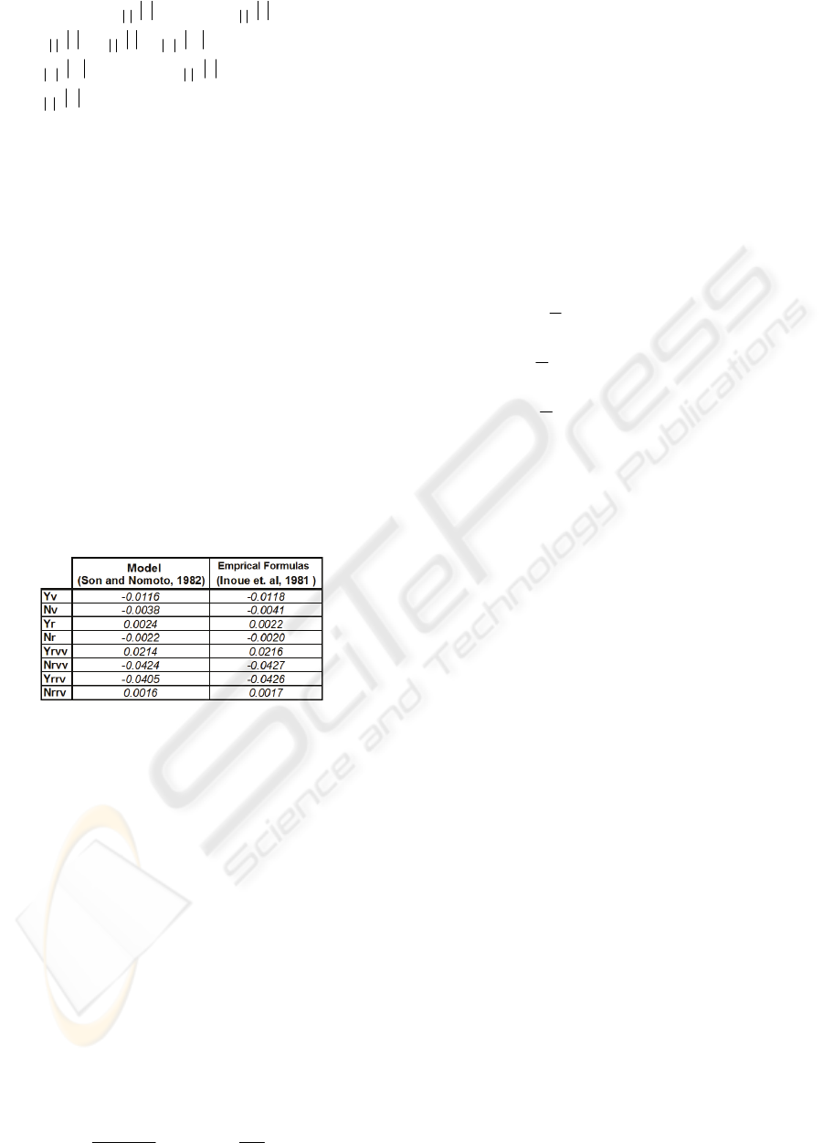
3 PHASE PLANE ANALYSIS
3.1 Phase Portrait of Course Keeping
Phase portraits of surface platform are shown. Yaw
angle (psi) versus its derivative yaw rate (r) in
Figure 2 and Roll angle versus roll rate in Figure 3
are used to obtain the phase portraits. If the real part
of the eigenvalues is positive, then x(t) and x(t) both
diverge to infinity, and the singularity point is called
an unstable focus.
Figure 2: The Phase Portrait (Yaw vs Yaw rate).
The phase portrait in Figure 3 demonstrates that
the unstable free motion of the surface platform.
Figure 3: The Phase Portrait(Roll angle vs Roll rate).
3.2 Phase Portrait of Zig Zag
Maneuver
It is intended that the surface platform makes zig-
zag maneuvers of 45° with a velocity of 8 m/s with
20° rudder angle. For a zig-zag maneuver, when the
angular acceleration plotted is against angular
velocity it shows how non-linear ship response can
be (Figure 4).
Figure 4: Phase Portrait of Zig Zag Maneuver.
4 LYAPUNOV STABILITY
THEOREM FOR SURFACE
PLATFORM DYNAMIC
A fully actuated surface platform can be described
by
() () ()MC D Bu
+
++==υυυυυg ητ

()J
=
ηηυ

where J(η) is singular for θ = ±90 degrees (Euler
angles), M= M
T
>0 and D(ν) = D
T
(ν) > 0. The
position is controlled by
1
( ) () ()
TT T
P
uBBB g J K
−
⎡
⎤
=
η− η η
⎣
⎦
where Kp = K
T
p > 0. Let
() ηηυυ
P
TT
KMV +=
2
1
be a Lyapunov function candidate for the closed-
loop system (4.1), (4.2) and (4.3). We take the time
derivative of the Lyapunov function candidate to
obtain
(
)
()
TT
P
VMJK
=
υυ+ηη


(
)
ηηηυυυυυ
P
TT
KJgDCBu )()()()( +−−−=
(
) υυυυυ )()( DC
T
−−=
υυυ )(D
T
−=
which is negative semidefinite. Asymptotic
stability can then be established by applying
LaSalle’s invariance principle, but the equilibrium
point (η, ν)=(0, 0) is only locally asymptotically
stable since J(η) is singular for θ = ±90 degrees.
MODELING, SIMULATION AND FEEDBACK LINEARIZATION CONTROL OF NONLINEAR SURFACE VESSELS
95

5 FEEDBACK LINEARIZATION
The basic idea with feedback linearization is to
transform the nonlinear systems dynamics into a
linear system (Freund (1973). Conventional control
techniques like pole placement and linear quadratic
optimal control theory can then be applied to the
linear system. Feedback linearization allows us to
design the controller directly based on a nonlinear
dynamic model that better describes a ship
maneuvering behavior. Consider Norrbin's nonlinear
ship steering equations of motion in the form
(Fossen 1992):
δψψψ =++
3
31

ddm
(16)
here m = T/K, d
1
= n
1
/K and d
3
= n
3
/K.
Taking the control law to be:
3
31
ˆˆ
ˆ
ψψδ
ψ

ddam ++=
(17)
where the hat denotes the estimates of the
parameters and a, can be interpreted as the
commanded acceleration, yields:
3
31
~
~
~
)( ψψψ
ψψ

ddamam ++=−
(18)
Here
mmm −=
ˆ
~
,
111
ˆ
~
ddd −=
and
333
ˆ
~
ddd −=
are the parameter errors. Consequently, the error
dynamics can be made globally asymptotically
stable by proper choices of the commanded
acceleration a
ψ
. (Fossen 1992) In the case of no
parametric uncertainties, equation (18) reduces to:
ψ
ψ
a=

which suggests that the commanded
acceleration should be chosen as:
ψ
ψ
ψ
ψ
~
~
pdd
KKa −−=

(19)
where
d
ψ
is the desired heading angle and
d
ψ
ψ
ψ
−=
~
is the heading error. This in turn yields
the error dynamics:
0
~
~
=++ ψψ
ψ
pd
KK

(20)
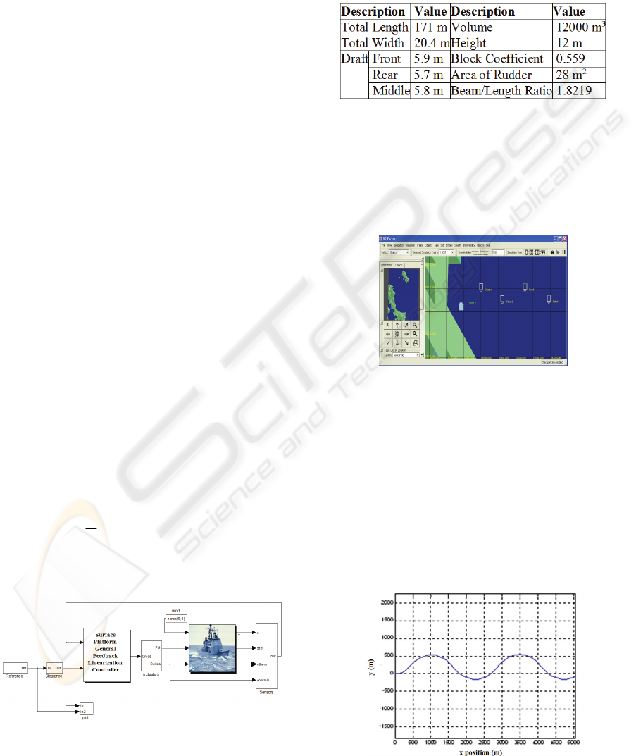
The block diagram of the control system is
shown in Figure 5.
Figure 5: Block Diagram of System.
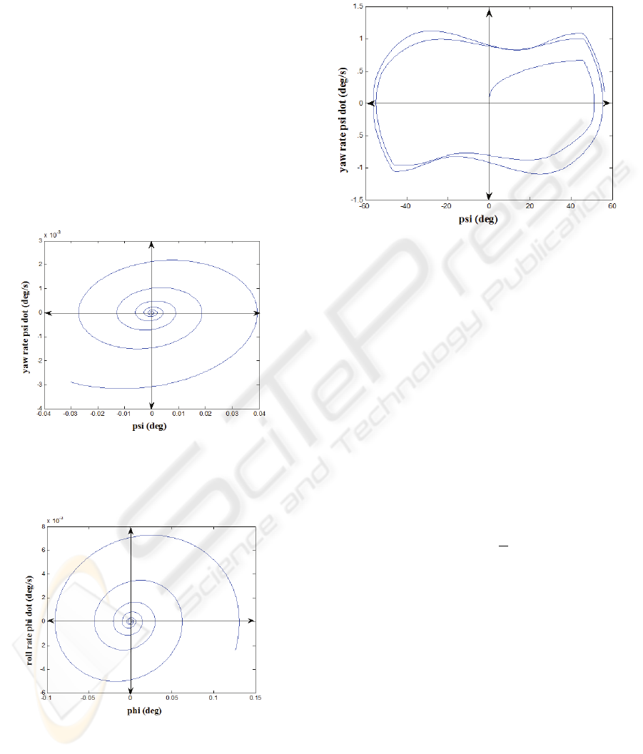
6 EXPERIMENTAL RESULTS
The crucial parameters of the surface platform
chosen for the illustration have been displayed in
Table 3.
Table 3: The main parameters of the surface platform.
In the sample application, it is intended that the
surface platform makes zig-zag maneuvers of 45°
with a velocity of 8 m/s. The route information
regarding this task is inputted by the VR-Forces
graphical user interface (Figure 6).The results below
have been produced after running the simulation for
800 seconds.
Figure 6: The route defined for the platform.
In this application, which is known as the zig zag
test of Kempf in the literature (Kempf, 1932), the
initial speed of the platform has been given as 0. The
platform is ordered to move to the specified
waypoints one by one by increasing its velocity up
to 8 m/s. It takes the platform 96 seconds to reach to
the first point. The first loop is accomplished in
approximately 295 seconds. The results are
acceptable for the motion behaviors that are
supposed to be realized by a large platform and
satisfactory in terms of simulation.
Figure 7: (a) Change of location.
ICINCO 2009 - 6th International Conference on Informatics in Control, Automation and Robotics
96

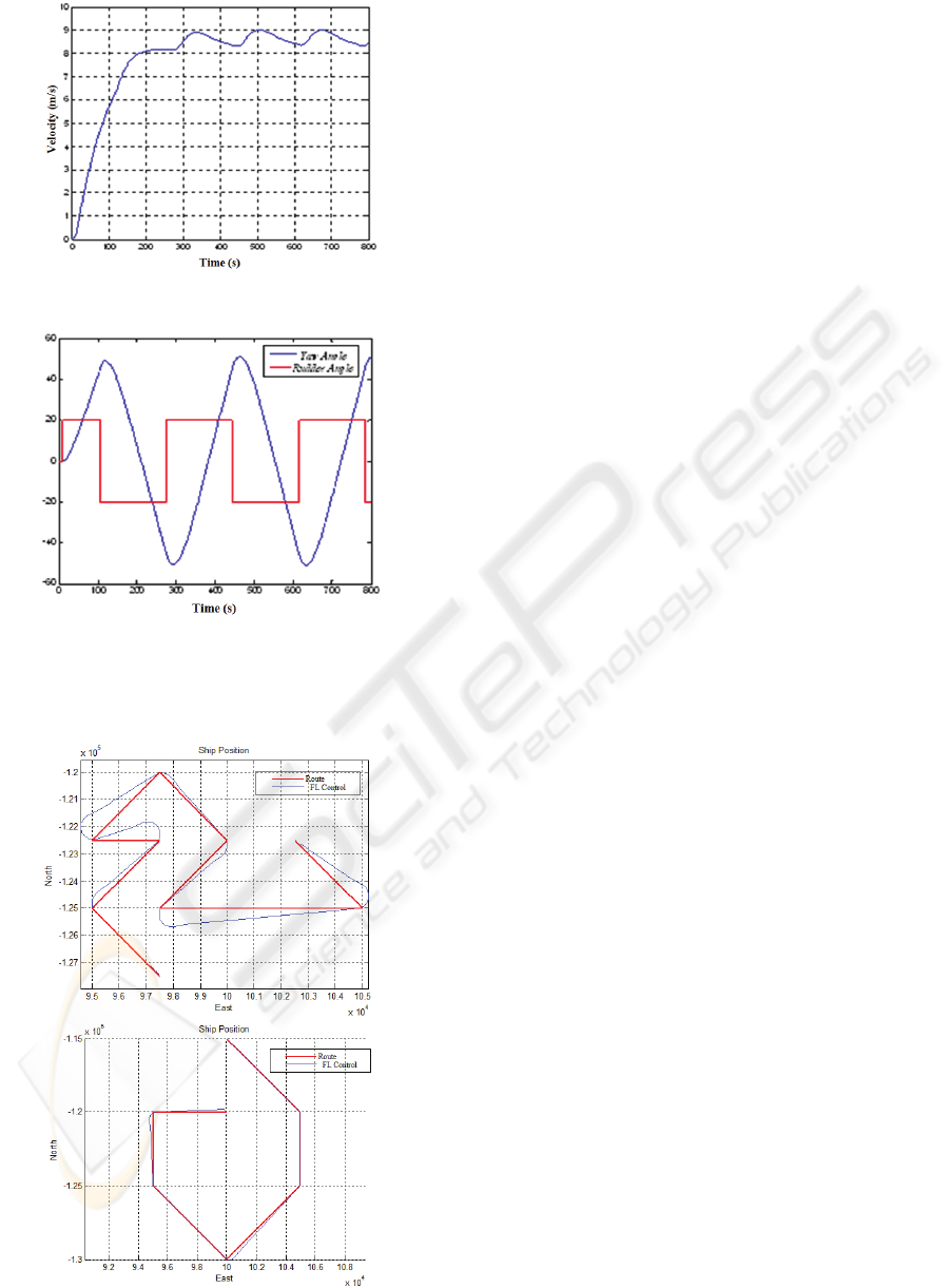
Figure 7: (b) Change of velocity.
Figure 8: Changes in the yaw angle and rudder angle of
the surface platform.
Controller performance can tried by some
different route applications:
Figure 9: Controller performance in different routes.
7 CONCLUSIONS
In this study, feedback linearization control has been
implemented in a nonlinear surface vessel model
including sea-state modeling (wave, current, wind).
The performance of the maneuver controller has
been illustrated through a simulation study. The
results are acceptable and satisfy for the needs of
military simulation. Although we have designed our
control to cover all influences, a more specified
design can upgrade the performance in each
different case. In the future work, the performance
of the controller may be compared with an
intelligent control technique.
REFERENCES
Abkowitz, M. A. , 1969. Stability and Motion Control of
Ocean Vehicles, M.I.T. Press, Cambridge,
Massachusetts.
Berteaux, H. O. , 1976. Buoy Engineering, Wiley and
Sons, New York.
Fossen, T. I., 1991. Nonlinear Modeling and Control of
Underwater Vehicles, Dr. Ing. thesis, Dept. of
Engineering Cybernetics, The Norwegian Institute of
Technology, Trondheim.
Fossen, T. I. and Paulsen, M. J., 1992. Adaptive Feedback
Linearization Applied to Steering of Ships,
Proceedings of the 1st IEEE Conference on Control
Applications (CCA'92), Dayton, Ohio, September 13-
16, 1992, pp. 1088-1093.
Freund, E., 1973. Decoupling and Pole Assignment in
Nonlinear Systems. Electronics Letter, No.16.
Inoue, S., Hirano, M., Kijima, K., 1981. Hydrodynamic
derivatives on ship manoeuvring; International Ship
Building Progress, Vol. 28.
Isherwood, R. M. , 1972. Wind Resistance of Merchant
Ships, RINA Trans., Vol. 115,pp. 327-338.
Kempf, G., 1932. Measurements of the Propulsive and
Structural Characteristics of Ships, Transactions of
SNAME, Vol. 40, pp. 42-57.
SNAME, 1950. The Society of Naval Architects and
Marine Engineers. Nomenclature for treating the
motion of submerged body through a fluid, Technical
Research Bulletin No. 1-5
MODELING, SIMULATION AND FEEDBACK LINEARIZATION CONTROL OF NONLINEAR SURFACE VESSELS
97