EXHIBITING PLANAR STRUCTURES FROM EGOMOTION
Samia Bouchafa, Antoine Patri and Bertrand Zavidovique
Institut d’Electronique Fondamentale, University Paris XI, 91405 Orsay Cedex, France
Keywords: Image motion analysis, Pattern recognition, Image scene analysis, Ego motion.
Abstract: This paper deals with plane extraction from a single moving camera through a new optical-flow cumulative
process. We show how this c-velocity defined by analogy to the v-disparity in stereovision, could serve
exhibiting any plane whatever their orientation. We focus on 3D-planar structures like obstacles, road or
buildings. A translational camera motion being assumed, the c-velocity space is then a velocity cumulative
frame in which planar surfaces are transformed into lines, straight or parabolic. We show in the paper how
this representation makes plane extraction robust and efficient despite the poor quality of classical optical
flow.
1 INTRODUCTION
Our work deals with obstacle detection from moving
cameras. In this application, most of real-time
implemented approaches are based on stereovision.
Yet stereo analysis shows two main drawbacks.
First, it tends to group objects which are close to
one-an-other. Second, height thresholds limit the
detection implying to miss small obstacles close to
the ground for example. Motion information is only
exploited afterwards for detected objects. Motion
analysis, on the other hand, allows the detection of
any moving object. Therefore, we propose to exploit
the ego-motion of the camera to distinguish between
various moving objects. To that aim, we have
established a correspondence with a very efficient
stereovision technique based on the v-disparity
concept (Labayrade, Aubert and Tarel, 2002). Our
conjecture is that such result is general. Thereby we
show how to extend the technique to detect planes
along an image sequence shot from a moving
vehicle. The apparent velocity from the scale change
occurring to image data takes place of the disparity
leading to the so-called c-velocity frame. In this
paper we propose a complete plane detection
process. Peculiar emphasis is placed on the
parabolas detection in the c-velocity space.
The paper is organized as follows: in the next
section we take a look at ego-motion based object
detection. Then we recall some pertaining relations
between 2D and 3D motion. The fourth part is
devoted to the computation of constant velocity
curves in the image plane – analogue in our c-
velocity frame of the lines of the v-disparity, and we
explain the cumulative process. The fifth section
details how parabolas – 3D planes – are extracted in
the c-velocity space using a Hough transform
enriched by a K-mean technique. After the section
devoted to results we conclude with discussions and
future work.
2 PREVIOUS WORK
Recent years have seen a profusion of work on 3D
motion, ego-motion or structure from motion
estimation using a moving camera. It was followed
by numerous classifications of existing methods
based on various criteria. A classification commonly
accepted groups existing techniques into three main
categories: discrete, continuous and direct
approaches.
- Discrete approaches (Hartley, 1995) are based
on matching and tracking primitives that are
extracted from image sequences (point, contour
lines, corners, etc.). They are usually very effective.
However, they suffer from a lack of truly reliable
and stable features, e.g. time and viewpoint
invariant. Moreover, in applications where the
camera is mounted on a moving vehicle,
homogeneous zones or linear marking on the ground
hamper the extraction of reliable primitives.
183
Bouchafa S., Patri A. and Zavidovique B. (2009).
EXHIBITING PLANAR STRUCTURES FROM EGOMOTION.
In Proceedings of the 6th International Conference on Informatics in Control, Automation and Robotics - Robotics and Automation, pages 183-188
DOI: 10.5220/0002194601830188
Copyright
c
 SciTePress

- Continuous approaches exploit optical flow
(MacLean, Jepson and Frecker, 1994). The
relationship between the computed optical flow and
real theoretical 3D motion allows - through
optimization techniques - to estimate the motion
parameters and depth at each point. Results are
dependent on the quality of the computed optical
flow.
- In direct approaches (Stein, Mano and Shashua,
2000), motion is determined directly from the
brightness invariance constraint without having to
calculate explicitly an optical flow. Motion
parameters are then deduced by conventional
optimization approaches.
- A large group of approaches (Irani, Rousso and
Peleg, 1997) - which can be indifferently discrete,
continuous or direct - exploits the parallax generated
by motion (motion parallax, affine motion parallax,
plane+parallax). These methods are based on the
fact that depth discontinuities make it doable to
separate camera rotation from translation. For
instance, in "Plane+parallax" approaches, knowing
the 2D motion of an image region where variations
in depth are not significant permits to eliminate the
camera rotation. Using the obtained residual motion
parallax, translation can be exhibited easily.
3 PRELIMINARIES
Consider a coordinate system O XYZ at the optical
centre of a pinhole camera, such that the axis OZ
coincides with the optical axis. We assume a
translational rigid straight move of the camera in the
Z direction. That does not restrict the generality of
computations. Moreover, the origin of the image
coordinates system is placed on the top left of the
image. If
00
(, )
x
y are the coordinates of the
principal point, then the ego-motion
(,)uv becomes:
() ()
00
and
zz
TT
uyyvxx
Z
Z
=− =−
The previous equations describe a 2D motion
field that should not be confused with optical flow
which describes the motion of observed brightness
patterns. We will assume here that optical flow is a
rough approximation of this 2D motion field. In
order to tackle the imprecision of optical flow
velocity vectors, we propose to define a Hough-like
projection space which – thanks to its cumulative
nature –allows performing robust plane detection.
4 NEW CONCEPT: C-VELOCITY
In stereovision, along a line of a stereo pair of
rectified images, the disparity is constant and varies
linearly over a horizontal plane in function of the
depth. Then, in considering the mode of the 2-D
histogram of disparity value vs. line index, i.e. the so
called v-disparity frame, the features of the straight
line of modes indicate the road plane for instance
(Labayrade, Aubert and Tarel, 2002). The
computation was then generalized to the other image
coordinate and vertical planes using the u-disparity
by several teams including ours on our autonomous
car.
In the same way we have transposed this concept
to motion. Our computations build on the fact that
any move of a camera results into an apparent shift
of pixels between images: that is disparity for a
stereo pair and velocity for an image sequence. The
v-disparity space draws its justification, after image
rectification that preserves horizontal – iso-disparity
– lines, from inverse-proportional relations between
first image horizontal-line positions vs. depth,
second depth vs. disparity. We show here under how
to exhibit the same type of relation in the ego-
motion case between
w (≅ disparity) and the iso-
velocity function index c (≅ line index v).
22 2 2
00
()()
(, ) (, )
z
T
uv yy xx
Z
Kfxy fxy c
K
=+= −+−
=× ⇒ = =
w
w
w
The translation
Z
T being that of the camera,
identical for all static points, if depth Z is constant
the iso-velocity curves are circles. c varies linearly
with the velocity vector. Beyond that “punctual”
general case, Z can be eliminated in considering
linear relations with (X,Y) i.e. plane surfaces well
fitting the driving application for instance.
4.1 The Case of a Moving Plane
Suppose now the camera is observing a planar
surface of equation (Trucco and Poggio, 1989):
T
d
=
nP , with
(,,)
x
yz
nnn=n
the unit normal to
the plane and d the distance "plane to origin". Let us
assume that the camera has a translational motion
(
)
0,0,
Z
T=T . We study four pertaining cases of
moving planes and establish the corresponding
motion field. a) Horizontal: road. b) Lateral:
buildings. c)Frontal
1
: fleeing or approaching
ICINCO 2009 - 6th International Conference on Informatics in Control, Automation and Robotics
184

obstacle, with
(0,0, )
o
Z
T=T
. d) Frontal
2
: crossing
obstacle, with
(,0,0)
o
X
T=T .
Normal
vector
Associated
3D motion
Dist. to the
origin
a)
(0,1,0)=n
()
0,0,
Z
T=T dist. d
r
b)
(1, 0, 0)=n
()
0,0,
Z
T=T dist. d
b
c)
(0,0,1)=n
()
0,0,
o
Z
Z
TT=+T dist. d
o
d)
(0,0,1)=n
(
)
,0,
o
XZ
TT=T
dist. d
o
The corresponding motion fields, after [2] for
instance, become those listed in the table below for
each case. Let
o
w
,
r
w
and
b
w
be
respectively the module of the apparent velocity of
an obstacle point, a road point and a building point.
We choose to group all extrinsic and intrinsic
parameters in a factor K and make it the unknown:
a)
00
2
0
()()
()
Z
r
Z
r
T
uyyxx
fd
T
vxx
fd
=−−
×
=−
×
b)
2
0
00
()
()()
Z
b
Z
b
T
uyy
fd
T
vyyxx
fd
=−
×
=−−
×
c)
0
0
()
()
o
ZZ
o
o
ZZ
o
TT
uyy
d
TT
vxx
d
+
=−
+
=−
d)
0
0
()
()
o
ZX
oo
Z
o
TTf
uyy
dd
T
vxx
d
=−−
=−
a)
422
000
()()()
r
K
xx yy xx=−+− −w
b)
422
000
()()()
r
K
yy yy x x=−+− −w
c)
22
00
()()
r
K
yy x x=−+−w
d)
Z
22
00
if T
( ) ( ) otherwise
o
oX
o
KT
Kx x yy
=
=−+−
w
w

Each type of
w leads to the corresponding
expression of c and then to the related iso-velocity
curve. For instance in the case of a building plane:
422
000
()()()cyyyyxx
K
==−+−+−
w
The final formula above proves that c is constant
along iso-velocity curves and proportional to
w ,
same as the disparity is proportional to the line value
v. Thus, as explained in introduction, the c-velocity
space will be a cumulative space that is constructed
in assigning to each pixel
(, )
x
y the corresponding c
value through the chosen model, and in
incrementing the resulting
()
,c w cell were w is
the velocity found in
(, )
x
y . The latter w is
computed thanks to a classical optical flow method.
A study of the function
(,)cxy that corresponds to
each plane model – in particular for the road and the
building model – led us to the following
conclusions: first, each previous curve intersects the
x axis (road model) or y axis (building model) in the
image plane in:
0
y
c± or
0
x
c± respectively.
Second, for a standard image size, the range of
variation of c is very large. For instance, for an
image size of 320×240:
max
32000c = (road model)
and 24000 (building model). As a consequence and
for implementation reasons, we propose to deal for
these two models with the relations between ||w|| and
c (see Figure 1).
Figure 1: The c-velocity space that depends on the chosen
relation between c and w: Linear for the obstacle model
and parabolic for the road and the building model.
4.2 Cumulative Curves
For each point (, )
x
yp= in the image, there is an
associated c value depending on the chosen plane
model (see left column of Figure 2). We can
calculate it once off-line because it only depends on
(, )
x
y . Also, it is possible for implementation
facilities and by analogy to image rectification (that
makes all epipolar lines parallel) to compute the
0 1 2 3 4 5
0
1
2
3
4
5
c
||w||
0 1 2 3 4 5
0
1
2
3
4
5
c
EXHIBITING PLANAR STRUCTURES FROM EGOMOTION
185

transformation that makes all the c-curves parallel to
the image line, that is the intensity function
(, )
I
cy
for road and obstacle model and
(,)
I
xc for building
model (see right column of Figure 2).
a) Obstacle model
b) Road model
c) Building model
Figure 2: Left: for each model, the corresponding c-values
for each point of the image. Right: images constructed
using the geometric transformation that makes all c-curves
parallel.
5 1D HOUGH TRANSFORM AND
K-MEAN CLUSTERING FOR
PARABOLAS EXTRACTION
Planes are represented in the c-velocity space by
parabolas that could be extracted using a Hough
transform. The distance p between each parabola
and its focus or its linea directrix is then cumulated
in a one dimensional Hough transform (see Figure
3). The classes of the histogram split by K-mean
clustering. Of course, any other clustering approach
could be applied.
()
()
2
2
1
44
c
wKc p
K
w
= ⇒ =− =−
0
5
10
15
20
25
30
1 22 43 64 85 106 127 148 169 190 211 232 253 274 295 316 337 358 379 400 421 442 463 484 505 526 547 568
Figure 3: Example of a 1D Hough transform on the c-
velocity space for detecting parabolas. For each (c,w) cell,
a p value is cumulated.
6 EXPERIMENTAL RESULTS
In Figure 4, we have considered an image sequence
in which one can see 6 moving planes: 2 planes
corresponding to buildings, 2 planes corresponding
to cars parked on the sides, a frontal moving
obstacle (a motorcycle crossing the road) and the
road plane. We have used the Lukas & Kanade
method for optical flow estimation (Lucas and
Kanade, 1981). In this sequence, velocity vectors are
in majority on vertical planes. In the building c-
velocity space, we get as expected 4 parabolas (see
Figure 4.b). We have studied in the effects of 3
kinds of perturbations that have a consequence on
the thickness of the parabolas. First, inter-model
perturbation, second the imprecision on optical flow
and third the possible pitch, yaw or roll of the
camera. We use 2 kinds of confidence factors. First
one is related to the translational motion hypothesis;
it is the difference Δ
foe
between the coordinate of
image centre and the position of the Focus of
expansion (for its estimation see section 6.1, results
on Figure 6). Second one is related to possible
contamination by planes of other models; it is the
variance σ of each K-mean class. Points far from the
mean belong probably to another plane model
(Figure 4.c).
ICINCO 2009 - 6th International Conference on Informatics in Control, Automation and Robotics
186

a) Top image: optical flow, here Δ
foe
=7. Bottom:
resulting vertical plane detection. Planes have a
label according to K-mean clustering
.
b) Resulting c-velocity for building model. Each
vote is normalized by the number of points in each
c-curve.
c) Results of parabolas extraction using a 1D
Hough transform followed by a K-mean clustering
(4 classes). In white the points that are discarded:
they probably belong to another plane model. σ
mean
= 10.
Figure 4: Example of results obtained from a database of
the French project “Love” (Logiciel d’Observation des
VulnérablEs).
Figure 5: Results of a building detection (top left image in
red). The crossing obstacle here is – as expected – not
detected in the building c-velocity space.
6.1 FOE Estimation
Several methods exist (Sazbon, Rotstein and Rivlin,
2004). For sake of further real on board
implementation, we favor here a method coherent
with the present computations. All pixels are asked
to vote for a global intersection point of apparent
velocity vectors within a regular Hough space.
Indeed, in the case of a translational motion, each
velocity vector with angle
θ
is directed toward the
FOE. Let us assume that
00
(, )
x
y are the FOE
coordinates in the image. Then we have:
11
0
0
tan tan
x
x
v
uyy
θ
−−
⎛⎞
−
⎛⎞
==
⎜⎟
⎜⎟
−
⎝⎠
⎝⎠
The above relation means that we can extract the
FOE by estimating the intersection of all velocity
vector lines. In practice, we have carried out a voting
space where each velocity vector votes for all the
points belonging to its support line. The FOE
corresponds then to the point with maximum votes.
EXHIBITING PLANAR STRUCTURES FROM EGOMOTION
187

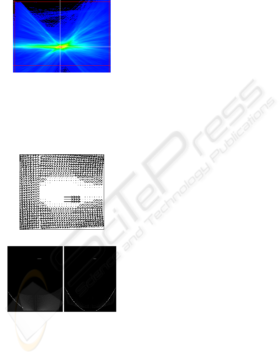
Figure 6: Voting space for FOE determination.
6.2 Results on Synthetic Images
In the following toy example, we generate a
synthetic velocity vectors field of a moving 3D
scene with 3 planes: a vertical one (on the left of the
image), an horizontal one (on the bottom of the
image) and a frontal plane with its own motion
parameters (a crossing obstacle), see Figure 7.a.
a) Velocity vectors field of a moving scene with a
building, a road and an obstacle plane.
b) Associated c-velocity spaces (left: building,
right: road). The parabolas indicate the expected
moving planes. The constant segment
corresponds to the obstacle; it appears in all the
c-velocity spaces because of its constant velocity.
Figure 7: Results on synthetic images.
The results confirm that this simulated ego-
motion (Figure 7,b) transforms a road plane and a
building plane into a parabola in the corresponding
c-velocity space. Likewise the obstacle in the middle
of the road is a segment with its own constant w.
7 CONCLUSIONS
First results are very encouraging and confirm that
the cumulative process is efficient in retrieving
major entities of a moving scene environment. Our
future work deals with implementing an iterative
approach that deals with all the c-velocity spaces.
Each detected plane from a given space could be
discarded from the other spaces in order to reduce
inter-model perturbation. On the other hand, we
propose to progressively generalize the approach to
more complex structures than planes and to more
complex motion models, including rotations for
instance.
REFERENCES
Hartley, R.I, 1995. In defense of the 8-point algorithm. In
Proc. IEEE Int. Conf. on Computer Vision,
Cambridge, MA, pp. 1064-1070.
Irani, M , Rousso, B, Peleg, S, 1997. Recovery of Ego-
Motion using region alignment. In IEEE Trans on
PAMI, vol. 19, n°3.
Labayrade, R, Aubert, D, Tarel, JP, 2002. Real Time
Obstacle Detection on Non Flat Road Geometry
through ‘V-Disparity’ Representation. In IEEE
Intelligent Vehicles Symposium 2002, Versailles, June
2002.
Lucas, B.D, Kanade, T, 1981. An Iterative Image
Registration Technique with an Application to Stereo
Vision (DARPA). In Proceedings of the 1981 DARPA
Image Understanding Workshop, pp. 121-130.
MacLean, W.J, Jepson, A.D , Frecker, R.C, 1994.
Recovery of egomotion and segmentation of
independant object motion using the EM algorithme.
In Proc. of the 5th British Machine Vision Conference,
pp. 13-16, York, U. K.
Sazbon, D, Rotstein, H, Rivlin, E, 2004. Finding the focus
of expansion and estimating range using optical flow
images and a matched filter. In MVA, vol. 15, n°4, pp.
229-236.
Stein, G. P , Mano, O, Shashua, A, 2000. A robust method
for computing vehicle ego-motion. In IEEE Intelligent
Vehicles Symposium, Dearborn, MI.
Trucco, E, Poggio, T, 1989. Motion field and optical flow:
qualitative properties. In IEEE Transactions on
Pattern Analysis Machine Intelligence, vol. 11, pp.
490-498.
ICINCO 2009 - 6th International Conference on Informatics in Control, Automation and Robotics
188