
A DECENTRALIZED COLLISION AVOIDANCE ALGORITHM FOR
MULTI-ROBOTS NAVIGATION
Michael Defoort, Arnaud Doniec and Noury Bouraqadi
Ecole de Mines de Douai, 941 rue Charles Bourseul, BP 10838, 59508 Douai, France
Keywords:
Decentralized intelligence, Real-time path planning, Collision avoidance, Receding horizon, Nonholonomic
mobile robots.
Abstract:
This paper presents a distributed strategy for the navigation of multiple autonomous robots. The proposed
planning scheme combines a decentralized receding horizon motion planner, in which each robot computes its
own planned trajectory locally, with a fast navigation controller based on artificial potential fields and sliding
mode control technique. This algorithm solves the collision avoidance problem. It explicitly accounts for
computation time and is decentralized, making it suited for real time applications. Simulation studies are
provided in order to show the effectiveness of the proposed approach.
1 INTRODUCTION
The research effort in multi-robots systems (MRS) re-
lies on the fact that multiple robots have the possibil-
ity to perform a mission more efficiently than a sin-
gle robot. Among all the topics of study in this field,
the issue of conflict resolution becomes an increas-
ingly important point. Many cooperative tasks such
as surveillance, search, rescue or area data acquisi-
tion need the robots to autonomously navigate with-
out collision.
Solving conflicts in MRS consists in introduc-
ing some coordination mechanisms in order to give
a coherence between the robot acts (Kuchar and
Yang, 2000). For motion planning, three coordination
mechanisms are identified:
• The Coordination by Adjustment, where each
robot adapts its behavior to achieve a common ob-
jective (Tomlin et al., 1998). However, most of the
planning algorithms are centralized, which often
limit their applicability in real systems.
• The Coordination by Leadership (or supervision)
where a hierarchical relationship exists between
robots (Das et al., 2002). Such an approach is easy
to implement. However, due to the lack of an ex-
plicit feedback from the followers to the leader,
the collision avoidance cannot be guaranteed if
followers are perturbed (during obstacle avoid-
ance for instance). Another disadvantage is that
the leader is a single point of failure.
• The Standardization where procedures are prede-
fined to solve some particular interaction cases
(Pallatino et al., 2007). While this approach can
lead to straightforward proofs, it also tends to be
less flexible with respect to changing conditions.
Here, the problem of interest is the decentralized
navigation for autonomous robots through a coordi-
nation by adjustment. Each vehicle is modeled as
an unicycle with a limited sensing range in order
to capture the essential properties of a wide range
of vehicles. They are dynamically decoupled but
have common constraints that make some conflicts.
Indeed, each robot has to avoid collision with the
other entities. Furthermore, the proposed framework
allows moving (and static) obstacles to be avoided
since they can be modeled as non cooperative enti-
ties.
Motion planning consists in generating a
collision-free trajectory from the initial to the final
desired positions for a robot. Since the environment
is partially known and further explored in real
time, the computation of complete trajectories from
start until finish must be avoided. Therefore, the
trajectories have to be computed gradually over time
while the mission unfolds. It can be accomplished
using an online receding horizon planner (Mayne
et al., 2000), in which partial trajectories from an
initial state toward the goal are computed by solving
optimal control problems over a limited horizon.
Two strategies for motion planning in MRS
44
Michael D., Doniec A. and Bouraqadi N. (2009).
A DECENTRALIZED COLLISION AVOIDANCE ALGORITHM FOR MULTI-ROBOTS NAVIGATION.
In Proceedings of the 6th International Conference on Informatics in Control, Automation and Robotics - Robotics and Automation, pages 44-51
DOI: 10.5220/0002194900440051
Copyright
c
SciTePress
are the centralized and decentralized (distributed)
approaches. Although the centralized one has been
used in different studies (see (Dunbar and Murray,
2002) for instance), its computation time which
scales exponentially with the number of robots, its
communication requirement and its lack of security
make it prohibitive. To overcome these limitations,
one can use a distributed strategy which results in be-
haviors closed to what is obtained with a centralized
approach. Recently, some decentralized receding
horizon planners have been proposed. In (Dunbar
and Murray, 2006), a distributed solution is provided
for the rigid formation stabilization problem.
In (Kuwata et al., 2006), the navigation problem is
solved through a coordination by leadership. Indeed,
the robots update their trajectory sequentially. In
(Defoort et al., 2007), a decentralized algorithm
based on a coordination by adjustment is proposed
to solve the navigation problem for MRS. However,
the large amount of information exchanged between
robots and the addition of several constraints make
this strategy prohibitive when the number of vehicles
increases.
One of other collision avoidance algorithm is
potential field method, where an artificial potential
function treats each robot as a charged particle
that repels all the other entities (Latombe, 1991;
De-Gennaro and Jadbabaie, 2006). However, most of
them are only based on relative position information
and do not consider coordination between coopera-
tive robots.
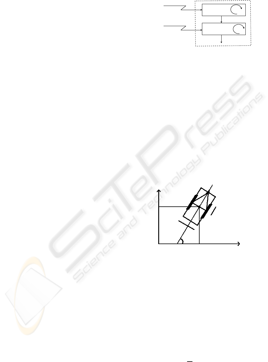
In this paper, we proposed a practical decentral-
ized scheme, based on a coordination by adjustment,
for real time navigation of large-scale MRS. As
illustrated in Fig. 1, the scheme consists of two
parallel processes:
• a distributed receding horizon planner, in which
each robot computes its own planned trajectory
locally, for the coordination between cooperative
robots,
• a reactive approach, which combines artificial po-
tential fields and sliding mode control technique,
for simultaneously tracking the planned trajectory
while avoiding collision with unexpected entities
(i.e. non cooperative entities).
The main advantages of the proposed strategy, espe-
cially for large-scale MRS, are the small amount of in-
formation exchanged between cooperative robots and
the robustness.
The outline of this paper is as follows. In Section
2, the problem setup is described. In Section 3, the
navigation algorithm is presented. Finally, numerical
results illustrate the effectiveness of the strategy.
Robot A
n
Receding horizon
planner
planned trajectory
real control inputs
Reactive navigation
controller
planned velocity
of cooperative robots
actual position and velocity
Process 1
Process 2
of non cooperative entities
actual position and velocity
(obstacles, moving objects)
Figure 1: Proposed navigation algorithm.
2 PROBLEM STATEMENT
2.1 Dynamic Model of the Robots
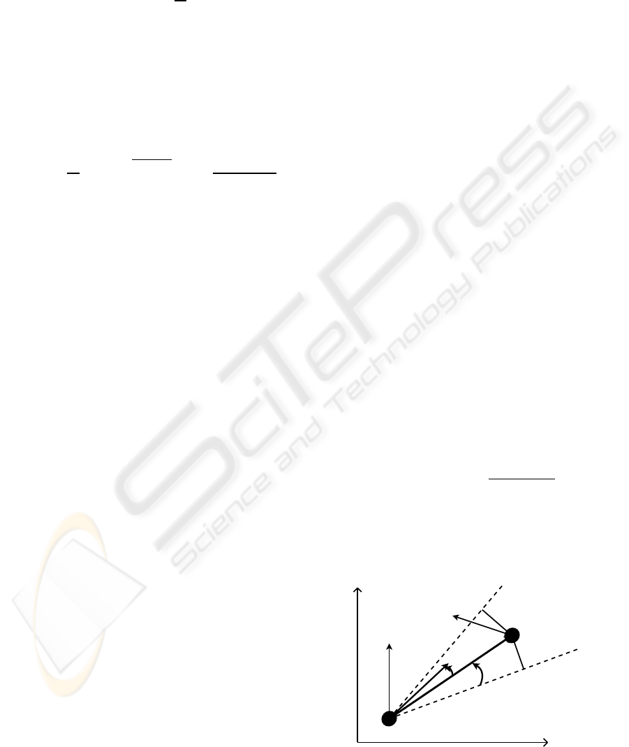
Each robot A
n
(n ∈ (1, ..., N) with N ∈ N), shown
in Fig. 2, is of unicycle-type. Its two fixed driving
wheels of radius r
n
, separated by 2ρ
n
, are indepen-
dently controlled by two actuators (DC motors) and
the passive wheel prevents the robot from tipping over
as it moves on a plane. Its configuration is given by:
η
η
η
n
= [x
n
,y
n
,θ
n
]
T
where (x
n
,y
n
) is the position of its mass center C
n
and
θ
n
is its orientation in the global frame.
y
n
x
n
θ
n
Y
C
n
j
Y
2ρ
n
r
n
Figure 2: Unicycle-type robot.
The dynamic model of robot A
n
is given as in (Do
et al., 2004):
˙
η
η
η
n
= J(η
η
η
n
)z
z
z
n
(1)
M
n
˙
z
z
z
n
+ D
n
z
z
z
n
= τ
τ
τ
n
(2)
where
• M
n
is a symmetric positive definite inertia matrix
• D
n
is a symmetric damping matrix
• the transformation matrix J(η
η
η
n
) is
J(η
η
η
n
) =
r
n
2
cosθ
n
cosθ
n
sinθ
n
sinθ
n
ρ
−1
n
−ρ
−1
n
(3)
A DECENTRALIZED COLLISION AVOIDANCE ALGORITHM FOR MULTI-ROBOTS NAVIGATION
45
• z
z
z
n
= [z
r
n
,z
l
n
]
T
where z
r
n
, z
l
n
are the angular veloci-
ties of the right and left wheels. The relationship
between z
z
z
n
and the linear and angular velocities,
denoted v
n
, w
n
, is
z
r
n
z
l
n
= B
n
v
n
w
n
with B
n
=
1
r
n
1 ρ
n
1 −ρ
n
(4)
• τ
τ
τ
n
= [τ
r
n
,τ
l
n
]
T
where τ
r
n
,τ
l
n
are the control torques
applied to the wheels of the robot
Remark 1. System (1)-(2) is flat (see (Fliess et al.,
1995) for details about flatness) since all system vari-
ables can be differentially parameterized by x
n
, y
n
as
well as a finite number of their time derivatives. For
instance, θ
n
, v
n
and w
n
can be expressed as
θ
n
= arctan
˙y
n
˙x
n
, v
n
=
q
˙x
2
n
+ ˙y
2
n
, w
n
=
¨y
n
˙x
n
− ¨x
n
˙y
n
˙x
2
n
+ ˙y
2
n
Remark 2. Speed u
u
u
n
= [ ˙x
n
, ˙y
n
]
T
of A
n
is restricted to
lie in a closed interval S
n
S
n
=
u
u
u
n
∈ R
2
| ku
u
u
n
k ≤ u
n,max
(5)
2.2 Assumptions and Control Objective
Assumption 1. The following assumptions are made:
• A
n
knows its position p
p
p
n
= [x
n
,y
n
]
T
and its veloc-
ity u
u
u
n
= [ ˙x
n
, ˙y
n
]
T
• A
n
has a physical safety area, which is centered
at C
n
with a radius R
n
, and has a circular com-
munication area which is also centered at C
n
with
a radius
¯
R
n
. Note that
¯
R
n
is strictly larger than
R
n
+ R
j
, j ∈ (1, .. ., N), j 6= n
• A
n
broadcasts (p
p
p
n
,u
u
u
n
) and receives (p
p
p
j
,u
u
u
j
)
broadcasted by other cooperative robots A
j
, in its
communication area
• A
n
can compute the relative position and velocity
(p
p
p
obs
i
,u
u
u
obs
i
) of non cooperative entities within a
given sensing range
• At the initial time t
ini
≥ 0, each robot starts at a
location outside of the safety areas of other enti-
ties
The objective is to find the control inputs τ
τ
τ
n
for
each robot A
n
such that, under Assumption 1,
• A
n
is stabilized toward its desired point p
p
p
n,des
, i.e.
lim
t→∞
kp
p
p
n
(t) − p
p
p
n,des
k = 0 (6)
• collisions are avoided
• all computations are done on board in a decentral-
ized cooperative way
Remark 3. It should be noted that for collision avoid-
ance, one can distinguish two kinds of entities, i.e.
• cooperative robots which are involved in a de-
tected potential collision
• non cooperative entities which cannot cooperate
in the collision avoidance process. They represent
the moving objects and static obstacles.
3 DISTRIBUTED ALGORITHM
In order to solve the multi-robots navigation problem,
a decentralized algorithm combining two parallel pro-
cesses is proposed. First, a receding horizon planner,
in which each robot computes its own planned trajec-
tory locally, achieves middle-term objectives, i.e. co-
ordination between cooperative robots which are in-
volved in a detected potential collision. Then, a reac-
tive navigation controller is proposed to fulfill short-
term objectives, i.e. trajectory tracking while taking
into account non cooperative entities.
3.1 Conflicts and Collisions
Definition 1. (conflict) A conflict occurs between two
cooperative robots A
n
and A
j
at time t
k
∈ R
+
if they
are not in collision at t
k
, but at some future time, a
collision may occur.
The following proposition, based on the well-
known concept of velocity obstacle (Fiorini and
Shiller, 1998), is useful to check the presence of con-
flicts.
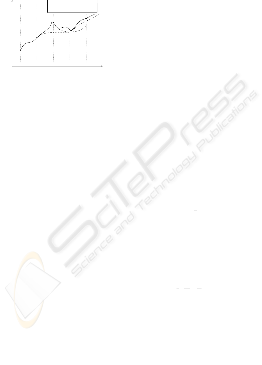
Proposition 1. Let us define for each pair (A
n
,A
j
),
the following variables depicted in Fig. 3:
β
nj
(t
k
) = arg(u
u
u
n
(t
k
) −u
u
u
j
(t
k
)) −arg(p
p
p
j
(t
k
) − p
p
p
n
(t
k
))
α
nj
(t
k
) = arcsin
R
n
+R
j
kp
p
p
j
(t
k
)−p
p
p
n
(t
k
)k
(7)
A necessary and sufficient condition for no conflict be-
tween A
n
and A
j
at t
k
is:
|β
nj
(t
k
)| ≥ α
nj
(t
k
) (8)
C
n
C
j
u
n
u
j
R
n
+ R
j
α
nj
β
nj
u
n
− u
j
Figure 3: Velocity obstacle concept.
ICINCO 2009 - 6th International Conference on Informatics in Control, Automation and Robotics
46

Definition 2. (conflict subset) For each A
n
, the con-
flict subset N
n
(t
k
) at time t
k
∈ R
+
is the set of all co-
operative robots which are in the communication area
of A
n
and in conflict with A
n
.
3.2 Receding Horizon Planner
The purpose of the distributed receding horizon plan-
ner is to decompose the overall problem into a family
of simple receding horizon planning problems which
are implemented in each robot A
n
.
In every problem, the same planning horizon T
p
∈
R
+
and update period T
c
∈ R
+
(T
c
< T
p
) are used.
The receding horizon updates are
t
k
= t
ini
+ (k − 1)T
c
, k ∈ N
∗
(9)
Remark 4. During the initialization step, that is to
say before robots move, we denote t
0
= t
ini
.
At each update t
k
, robots in conflict exchange in-
formation about each others (position, velocity, .. .).
Then, in parallel, every robot A
n
computes an antic-
ipated trajectory, denoted
b
p
p
p
j
(t,t
k
) and an anticipated
velocity
b
u
u
u
j
(t,t
k
), over the overall horizon, for all A
j
belonging to N
n
(t
k
). These trajectories are obtained
without taking the collision avoidance constraint into
account. Therefore, by design, the anticipated trajec-
tory is the same in every receding horizon planning
problem in which it occurs. At last, in parallel, ev-
ery robot A
n
computes only its own planned trajec-
tory p
p
p
∗
n
(t,t
k
) and planned velocity u
u
u
∗
n
(t,t
k
), over the
planning horizon T
p
, in order to integrate the colli-
sion avoidance between cooperative robots. From the
planned trajectory and velocity associated to the plan-
ning horizon T
p
, only the part which corresponds to
the update horizon T
c
is stored.
Remark 5. Note that the first argument of p
p
p
∗
n
,
b
p
p
p
n
,
u
u
u
∗
n
and
b
u
u
u
n
denotes time. The second argument is only
added to distinguish at which receding horizon update
the trajectory and velocity are computed.
The collection of distributed receding horizon
planning problems is formally defined as Problems 1-
2 for each robot A
n
.
Problem 1. For each robot A
n
and at any update t
k
,
k ∈ N:
Given
: the actual positions p
p
p
n
(t
k
), p
p
p
j
(t
k
) and the ac-
tual velocities u
u
u
n
(t
k
), u
u
u
j
(t
k
) of robot A
n
and robots A
j
belonging to N
n
(t
k
), respectively.
Find
: the anticipated trajectory and velocity pairs
(
b
p
p
p
i
(t,t
k
),
b
u
u
u
i
(t,t
k
)), ∀i ∈
i ∈ N | A
i
∈ N
n
(t
k
) ∪ {A
n
}
subject to the following constraints:
b
p
p
p
i
(t
k
,t
k
) = p
p
p
i
(t
k
)
b
u
u
u
i
(t
k
,t
k
) = u
u
u
i
(t
k
)
b
u
u
u
i
(t,t
k
) ∈ S
i
, ∀t ≥ t
k
(10)
The anticipated trajectories are computed without
taking the collision avoidance constraint into account.
That is why, to integrate the path planning with local
collision avoidance, the following problem is solved.
Problem 2. For each robot A
n
and at any update t
k
,
k ∈ N:
Given
: the anticipated pairs (
b
p
p
p
i
(t,t
k
),
b
u
u
u
i
(t,t
k
)), ∀i ∈
i ∈ N | A
i
∈ N
n
(t
k
) ∪ {A
n
}
.
Find
: the planned trajectory and velocity pairs
(p
p
p
∗
n
(t,t
k
),u
u
u
∗
n
(t,t
k
)) that minimizes
Z
t
k+1
+T
p
t
k+1
a
n
∑
j
b
U
nj,rep
(t) + kp
p
p
∗
n
(t,t
k
) −
b
p
p
p
n
(t,t
k
)k
!
dt
(11)
subject to the following constraints:
p
p
p
∗
n
(t
k+1
,t
k
) = p
p
p
∗
n
(t
k+1
,t
k−1
)
u
u
u
∗
n
(t
k+1
,t
k
) = u
u
u
∗
n
(t
k+1
,t
k−1
)
u
u
u
∗
n
(t,t
k
) ∈ S
n
, ∀t ∈
t
k+1
,t
k+1
+ T
p
(12)
where
b
U
nj,rep
(t) =
(
0 if
b
ρ
nj
(t) ≥ b
n
1
2
1
b
ρ
nj
(t)
−
1
b
n
2
else
b
ρ
nj
(t) = kp
p
p
∗
n
(t,t
k
) −
b
p
p
p
j
(t,t
k
)k −(R
n
+ R
j
)
(13)
a
n
and b
n
are strictly positive factors which can vary
among robots to reflect differences in aggressiveness
(a
n
< 1, b
n
≪ 1) and shyness (a
n
> 1, b
n
≫ 1).
One can note that the first part of cost (11) is de-
signed to enforce the collision avoidance between co-
operative robots. The cost term kp
p
p
∗
n
(t,t
k
) −
b
p
p
p
n
(t,t
k
)k
in (11) is a way of penalizing the deviation of the
planned trajectory p
p
p
∗
n
(t,t
k
) from the anticipated tra-
jectory
b
p
p
p
n
(t,t
k
), which is the trajectory that other
robots rely on. In previous work, this term was incor-
porated into the decentralized receding horizon plan-
ner as a constraint (Defoort et al., 2007). The formu-
lation presented here is an improvement over this past
formulation, since the penalty yields an optimization
problem that is much easier to solve.
Remark 6. One can note that constraints (12) which
guarantee the continuity of the planned trajectory and
velocity need p
p
p
∗
n
(t
k+1
,t
k−1
) and u
u
u
∗
n
(t
k+1
,t
k−1
) com-
puted in the previous step. Therefore, the proposed
planner is not able to reject external disturbances or
inherent discrepancies between the model and the real
process. However, it takes the real time constraint
into account. Indeed, each robot has a limited time
to plan its trajectory. The time allocated to make its
decision depends on its perception sensors, its com-
putation delays and is less than the update period T
c
(see Fig. 4).
The discussed claim for robustness in trajectory track-
ing will be achieved hereafter.
A DECENTRALIZED COLLISION AVOIDANCE ALGORITHM FOR MULTI-ROBOTS NAVIGATION
47
t
k
t
k+1
Anticipated trajectory
Planned trajectory
p
∗
n
(t, t
k−1
)
p
∗
n
(t, t
k
)
p
∗
n
(t, t
k
)
Comput.
of
Comput.
of
p
∗
n
(t, t
k+1
)
Figure 4: Implementation of the receding horizon planner.
Remark 7. A compromise must be done between re-
activity and computation time. Indeed, the planning
horizon must be sufficiently small in order to have
good enough results in terms of computation time.
However, it must be higher than the update period to
guarantee enough reactivity.
Remark 8. To numerically solve Problems 1-2, a
nonlinear trajectory generation algorithm (Defoort
et al., 2009) is applied. It is based on finding tra-
jectory curves in a lower dimensional space and pa-
rameterizing these curves by B-splines. A constrained
feasible sequential quadratic optimization algorithm
is used to find the B-splines coefficients that optimize
the performance objective while respecting the con-
straints.
3.3 Reactive Navigation Controller
Hereafter, a reactive approach, which combines arti-
ficial potential fields and sliding mode control tech-
nique, for simultaneously tracking the planned trajec-
tory while avoiding collision with unexpected entities
(i.e. non cooperative entities), is proposed.
Since the robot dynamics (1)-(2) is of strict feed-
back systems (see (Krstic et al., 1995) for details
about strict feedback systems) with respect to the
robot linear and angular velocities (i.e. v
n
and w
n
), a
backstepping procedure is used to design the control
input τ
τ
τ
n
. That is why the control design is divided
into two main steps.
3.3.1 Step 1 based on Artificial Potential Fields
Let us introduce the following notations:
θ
ne
= θ
n
− γ
θ
n
v
ne
= v
n
− γ
v
n
(14)
where γ
θ
n
and γ
v
n
are auxiliary variables used to avoid
collisions. Replacing expressions (14) into the first
two equations of (1) and using (4) yield:
˙
p
p
p
n
=
cosγ
θ
n
sinγ
θ
n
γ
v
n
+ ∆
1n
+ ∆
2n
(15)
with ∆
1n
= γ
v
n
(cosθ
ne
− 1)cosγ
θ
n
− sinθ
ne
sinγ
θ
n
sinθ
ne
cosγ
θ
n
+ (cosθ
ne
− 1)sinγ
θ
n
and ∆
2n
= v
ne
cosθ
n
sinθ
n
.
The objective is to design the auxiliary variables
γ
v
n
and γ
θ
n
such that robot A
n
robustly tracks its
planned trajectory p
p
p
∗
n
while avoiding unexpected col-
lisions. Here, artificial potential functions are used in
order to design an attractive force between the robot
and its planned trajectory and a repulsive force to
avoid collisions.
In conventional potential field method (Latombe,
1991), the planned robot velocity u
u
u
∗
n
is assumed to
be zero and the obstacle velocity u
u
u
obs
i
is not consid-
ered. However, to make robot A
n
track the planned
trajectory among moving obstacles, velocities u
u
u
∗
n
and
u
u
u
obs
i
play key roles. This issue will be addressed
by extending the results given in (Huang, 2009).
Let us consider the conventional potential function
(Latombe, 1991):
U
n
= U
n,att
+U
n,rep
(16)
where U
n,att
and U
n,rep
are, respectively, the attractive
potential defined to track the planned trajectory p
p
p
∗
n
and the repulsive potential related to collision avoid-
ance, specified as follows:
• The attractive potential is designed such that it
puts penalty on the tracking error and is equal to
zero when the robot is at its desired position, i.e.
U
n,att
=
1
2
kp
p
p
n
− p
p
p
∗
n
k
2
(17)
• The repulsive potential is designed such that it
equals to infinity when a collision occurs with A
n
and decreases according to the relative distance
between A
n
and an obstacle, i.e.
U
n,rep
= c
n
∑
i
U
ni,rep
(18)
with
U
ni,rep
=
(
0 if ρ
ni
≥ d
n
1
2
1
ρ
ni
−
1
d
n
2
else
(19)
where
ρ
ni
is the minimum distance between robot A
n
and
the obstacle i. c
n
and d
n
are strictly positive fac-
tors which have similar properties as a
n
and b
n
.
Proposition 2. If the errors θ
ne
and v
ne
are asymptot-
ically stable, A
n
robustly tracks its planned trajectory
p
p
p
∗
n
while avoiding collisions using the auxiliary vari-
ables:
γ
v
n
=
[(ku
u
u
∗
n
kcos(θ
∗
n
− ψ
n
) − c
n
∑
i
ξ
ni
ku
u
u
obs
i
kcos(θ
obs
i
− ψ
ni
)
+kp
p
p
n
− p
p
p
∗
n
k)
2
+ ku
u
u
∗
n
k
2
sin
2
(θ
∗
n
−
¯
ψ
n
)]
0.5
γ
θ
n
=
¯
ψ
n
+ arcsin
ku
u
u
∗
n
k sin(θ
∗
n
−
¯
ψ
n
)
γ
v
n
(20)
ICINCO 2009 - 6th International Conference on Informatics in Control, Automation and Robotics
48

with
θ
∗
n
= arg(u
u
u
∗
n
)
θ
obs
i
= arg(u
u
u
obs
i
)
ψ
n
= arg(p
p
p
∗
n
− p
p
p
n
)
ψ
ni
= arg(p
p
p
obs
i
− p
p
p
n
)
¯
ψ
n
= arctan
sinψ
n
−c
n
∑
i
ξ
ni
sinψ
ni
cosψ
n
−c
n
∑
i
ξ
ni
cosψ
ni
ξ
ni
=
(
0 if ρ
ni
≥ d
n
1
ρ
ni
−
1
d
n
1
(ρ
ni
)
2
1
kp
p
p
n
−p
p
p
∗
n
k
else
Proof. Let us differentiate U
n
with respect to time in
equation (16), i.e.:
˙
U
n
=
˙
U
n,att
+
˙
U
n,rep
(21)
Substituting (20) into (21) yields after some geomet-
ric manipulations:
˙
U
n
= kp
p
p
∗
n
− p
p
p
n
k(ku
u
u
∗
n
kcos(θ
∗
n
− ψ
n
) − γ
v
n
cos(γ
θ
n
− ψ
n
)
−c
n
∑
i
ξ
ni
ku
u
u
obs
i
kcos(θ
obs
i
− ψ
ni
) + γ
v
n
cos(γ
θ
n
− ψ
ni
)
)
+
(p
p
p
n
− p
p
p
∗
n
)
T
− c
n
∑
i
ξ
ni
kp
p
p
n
−p
p
p
∗
n
k
kp
p
p
n
−p
p
p
obs
i
k
(p
p
p
n
− p
p
p
obs
i
)
T
(∆
1n
+ ∆
2n
)
= kp
p
p
∗
n
− p
p
p
n
k(ku
u
u
∗
n
kcos(θ
∗
n
− ψ
n
) − γ
v
n
cos(γ
θ
n
−
¯
ψ
n
)
−c
n
∑
i
ξ
ni
ku
u
u
obs
i
kcos(θ
obs
i
− ψ
ni
)
)
+
(p
p
p
n
− p
p
p
∗
n
)
T
− c
n
∑
i
ξ
ni
kp
p
p
n
−p
p
p
∗
n
k
kp
p
p
n
−p
p
p
obs
i
k
(p
p
p
n
− p
p
p
obs
i
)
T
(∆
1n
+ ∆
2n
)
= kp
p
p
∗
n
− p
p
p
n
k(ku
u
u
∗
n
kcos(θ
∗
n
− ψ
n
) −
q
γ
2
v
n
− ku
u
u
∗
n
k
2
sin
2
(θ
∗
n
−
¯
ψ
n
)
−c
n
∑
i
ξ
ni
ku
u
u
obs
i
kcos(θ
obs
i
− ψ
ni
)
)
+
(p
p
p
n
− p
p
p
∗
n
)
T
− c
n
∑
i
ξ
ni
kp
p
p
n
−p
p
p
∗
n
k
kp
p
p
n
−p
p
p
obs
i
k
(p
p
p
n
− p
p
p
obs
i
)
T
(∆
1n
+ ∆
2n
)
Assuming that the errors θ
ne
and v
ne
are asymptoti-
cally stable (i.e. ∆
1n
= ∆
2n
= 0), one can get from
(20):
˙
U
n
≤ −kp
p
p
∗
n
− p
p
p
n
k
2
(22)
Since U
n
≥ 0 and
˙
U
n
≤ 0, U
n
is bounded. That is
why A
n
robustly tracks its planned trajectory p
p
p
∗
n
while
avoiding collisions.
3.3.2 Step 2 based on Sliding Mode Technique
Now, the objective is to force the motion of robot A
n
such that the errors θ
ne
and v
ne
are asymptotically sta-
ble. The proposed strategy is based on the so-called
second order sliding mode control (SMC) approach.
The SMC methodology (Utkin et al., 1999) is cho-
sen because it is a robust technique to control non-
linear systems operating under uncertainty conditions
(Fridman and Levant, 2002). Furthermore, second or-
der SMC can reduce the chattering phenomenon (high
frequency vibrations of the controlled system which
degrade the performances). Indeed, instead of influ-
encing the first sliding variable time derivative, the
signum function acts on its second time derivative.
This method can also achieve a better convergence
accuracy with respect to discrete sampling time than
conventional SMC (see (Fridman and Levant, 2002)
for a survey).
Let us apply to system (1)-(2) the following pre-
liminary feedback:
¯
τ
τ
τ
n
= (M
n
B
n
)
−1
(τ
τ
τ
n
− D
n
z
z
z
n
) (23)
where
¯
τ
τ
τ
n
= [
¯
τ
1n
,
¯
τ
2n
]
T
is the auxiliary control input.
Thus, system (1)-(2) can be expressed as follows:
˙
η
η
η
n
= J(η
η
η
n
)B
n
v
n
w
n
(24)
˙v
n
˙w
n
=
¯
τ
τ
τ
n
(25)
Since the relative degree of system (24)-(25) with
respect to the sliding variable v
ne
is only one, a dy-
namic extension is done before designing the control
(see (Isidori, 1989) for further details). Thus, an inte-
grator chain is added on the input variable
¯
τ
1n
.
There are several algorithms to ensure the finite
time stabilization of the sliding variables θ
ne
and v
ne
towards the origin. Among them, the sampled twist-
ing algorithm (Fridman and Levant, 2002) has been
developed for systems with relative degree two. This
algorithm provides good convergence accuracy and
robustness properties. It does not require the knowl-
edge of the time derivative of the sliding variables and
takes into account some practical constraints such as
the sampling of the measurement and the control.
Proposition 3. Consider system (1)-(2). The errors
θ
ne
and v
ne
are stable in finite time under the nonlin-
ear controller defined in (23) where
˙
¯
τ
1n
=
−λ
1,M
sign(θ
ne
) if θ
ne
∆
θ
ne
> 0
−λ
1,m
sign(θ
ne
) if θ
ne
∆
θ
ne
≤ 0
¯
τ
2n
=
−λ
2,M
sign(v
ne
) if v
ne
∆
v
ne
> 0
−λ
2,m
sign(v
ne
) if v
ne
∆
v
ne
≤ 0
(26)
with
∆
θ
ne
=
0 if k = 0
θ
ne
(kT
s
) − θ
ne
((k− 1)T
s
) else
∆
v
ne
=
0 if k = 0
v
ne
(kT
s
) − v
ne
((k− 1)T
s
) else
(27)
T
s
is the sampling period, k ∈ N is related to the time
of the process and λ
i,m
, λ
i,M
, i = 1,2 are positive con-
stants high enough to enforce the sliding motion.
Proof. It can be shown that this controller ensures
a finite time convergence of the trajectories onto
the manifold {v
ne
= ˙v
ne
= 0} and
θ
ne
=
˙
θ
ne
= 0
(see (Fridman and Levant, 2002) for further details).
Hence, the application of the control input (26) re-
sults in the robust finite time stabilization of θ
ne
and
v
ne
.
Remark 9. We would like to emphasize that although
not explicitly considered here the procedure based
on sliding mode control guarantees proper behavior
even in the presence of uncertainties in the mass and
inertia of the robots and additive disturbances to the
linear and angular velocities which constitute very re-
alistic assumptions.
A DECENTRALIZED COLLISION AVOIDANCE ALGORITHM FOR MULTI-ROBOTS NAVIGATION
49
Once the sliding mode occurs on all the surfaces
(which happens in finite time), based on Proposition
2, the global control objectives, defined in Section
2.2, are fulfilled.
Some specific advantages of the proposed decentral-
ized algorithm are enumerated below:
• robustness with respect to uncertainties and dis-
turbances (sliding mode controller),
• reactivity (potential field functions),
• low communication bandwidth, i.e. small amount
of information is locally exchanged,
• reduction of deadlocks due to local minima in po-
tential field (anticipation and coordination mech-
anism through the receding horizon planner).
4 SIMULATION RESULTS
This section demonstrates the performance of the pro-
posed decentralized algorithm. The following simula-
tions showcase two different scenarios for which the
environment is partially known (i.e. the range of sen-
sors of each robot is of radius 1.5m).
The main parameters of the robots are: ∀n, R
n
=
0.25m,
¯
R
n
= 4m and u
n,max
= 1m/s. For the decen-
tralized algorithm, the following parameters are used:
T
p
= 3s, T
c
= 0.5s, a
n
= c
n
= 1, b
n
= 2, d
n
= 0.5,
λ
1,M
= λ
2,M
= 10, λ
1,m
= λ
2,m
= 1 and T
s
= 0.01s.
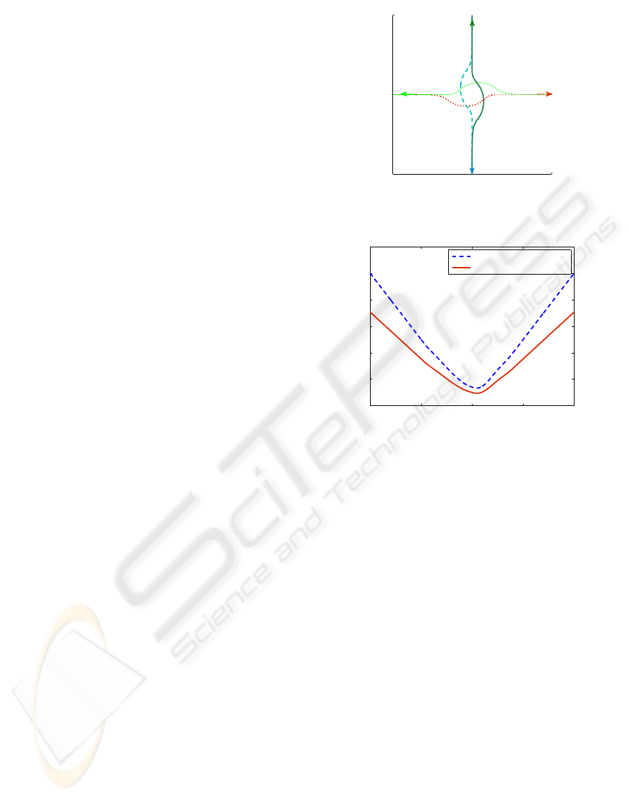
4.1 Scenario 1: Crossing
In this scenario, there are four robots (N = 4) start-
ing at p
p
p
1
(t
ini
) = [5,0]
T
, p
p
p
2
(t
ini
) = [15, 0]
T
, p
p
p
3
(t
ini
) =
[10,5]
T
and p
p
p
4
(t
ini
) = [10,− 5]
T
respectively, with ve-
locities equal to zero. These robots must cross each
other in order to reach their desired configuration
p
p
p
1,des
= [15,0]
T
, p
p
p
2,des
= [5,0]
T
, p
p
p
3,des
= [10,−5]
T
and p
p
p
4,des
= [10,5]
T
. One can note that this problem
is not trivial due to its symmetry properties.
The simulation results are given in Fig. 5. One
can see that each robot modifies its trajectory in order
to avoid collision. Figure 5(b) depicts the evolution
of the distance between robots. Since it is higher than
0.5m, the collision avoidance is guaranteed.
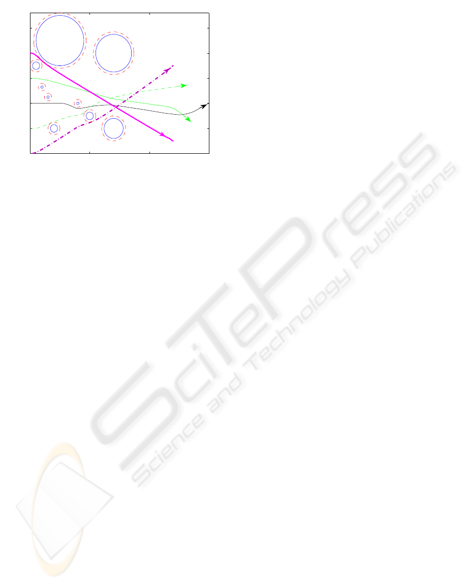
4.2 Scenario 2: Reconfiguration with
Collision Avoidance
In this scenario, a swarm of five robots (N = 5) recon-
figures its geometric shape (from “linear” to “triangu-
lar”) while avoiding collisions with obstacles. The
5 10 15
−5
0
5
x(m)
y(m)
A
3
A
4
A
2
A
1
(a)
0 5 10 15 20
0
2
4
6
8
10
12
t(s)
(m)
p
1
− p
2
p
1
− p
3
= p
1
− p
4
(b)
Figure 5: Four vehicles simulation: (a) Robot trajectories.
(b) Relative distances between A
1
and other robots.
proposed decentralized controller has only a limited
knowledge of the obstacles (initially unknown). It
simply keeps the robots spaced out using the proposed
potential field technique. The five robots make deci-
sions in order to avoid collisions. One can note that
the number of potential conflicts is high.
One can see in Fig. 6 that under the proposed de-
centralized algorithm, the robots meet the objective
defined in Section 2.2. Note that the radius of obsta-
cles is increased by 0.25m (dotted lines around obsta-
cles) to take the size of robots into account.
5 CONCLUSIONS
A new distributed strategy for the navigation of mul-
tiple autonomous robots is presented. The pro-
posed scheme combines a decentralized receding
horizon motion planner to satisfy middle-term objec-
tives (coordination between cooperative robots) with
a fast navigation controller based on artificial poten-
tial fields and sliding mode control technique to sat-
isfy short-term objectives (collision avoidance and
ICINCO 2009 - 6th International Conference on Informatics in Control, Automation and Robotics
50
0 5 10
−4
−2
0
2
4
6
x (m)
y (m)
A
1
A
2
A
3
A
5
obstacle
obstacle
obstacle
A
4
Figure 6: Collision avoidance of five robots.
trajectory tracking). The fact that there is no leader
increases the security and the robustness of the mis-
sions. Simulation studies are provided in order to
show the effectiveness of the proposed approach.
Experimental testing on WifiBot is under way. In
the future, it is planned to design real time observers
to estimate the relative velocities between robots.
REFERENCES
Das, A., Fierro, R., Kumar, V., Ostrowski, J., Spetzer, J.,
and Taylor, C. (2002). A vision-based formation con-
trol framework. IEEE T. Robotic Autom., 18(5):pp.
813–825.
De-Gennaro, M. and Jadbabaie, A. (2006). Formation con-
trol for a cooperative multi-agent system using decen-
tralized navigation functions. In American Control
Conf.
Defoort, M., Floquet, T., Kokosy, A., and Perruquetti, W.
(2007). Decentralized robust control for multi-vehicle
navigation. In European Control Conf.
Defoort, M., Palos, J., Kokosy, A., Floquet, T., and Perru-
quetti, W. (2009). Performance based reactive nav-
igation for nonholonomic mobile robots. Robotica,
27(2):pp. 281–290.
Do, K., Jiang, Z., and Pan, J. (2004). A global output-
feedback controller for simultaneous tracking and sta-
bilization of unicycle-type mobile robots. IEEE T. Au-
tomat. Contr., 20(3):pp. 589–594.
Dunbar, W. and Murray, R. (2002). Model predictive con-
trol of coordinated multi-vehicle formation. In IEEE
Conf. on Decision and Control.
Dunbar, W. and Murray, R. M. (2006). Distributed receding
horizon control for multi-vehicle formation stabiliza-
tion. Automatica, 42(4):pp. 549–558.
Fiorini, P. and Shiller, Z. (1998). Motion planning in dy-
namic environments using velocity obstacles. Int. J.
Robot. Res., 17(7):pp. 760–772.
Fliess, M., Levine, J., Martin, P., and Rouchon, P. (1995).
Flatness and defect of nonlinear systems: introductory
theory and examples. Int. J. Control, 61(6):pp. 1327–
1361.
Fridman, L. and Levant, A. (2002). Higher order sliding
mode modes. Sliding mode control in Engineering,
Ed W. Perruquetti, J. P. Barbot, pages 53–101.
Huang, L. (2009). Velocity planning for a mobile robot
to track a moving target - a potential field approach.
Robot. Auton. Syst., 57(1):pp. 55–63.
Isidori, A. (1989). Nonlinear control systems. Springer,
New York, 2nd edition.
Krstic, M., Kanellakopoulos, I., and Kokotovic, P. (1995).
Nonlinear and adaptative control design. Wiley, N. Y.
Kuchar, J. and Yang, L. (2000). A review of conflict detec-
tion and resolution modeling methods. IEEE T. Intell.
Transp., 1(4):pp. 179–189.
Kuwata, Y., Richards, A., Schouwenaraars, T., and How, J.
(2006). Decentralized robust receding horizon con-
trol. In American Control Conf.
Latombe, J. (1991). Robot Motion Planning. Kluwer Aca-
demic Publishers, Norwell, MA.
Mayne, D., Rawlings, J., Rao, C., and Scokaert, P. (2000).
Constrained model predicitive control: Stability and
optimality. Automatica, 36(6):pp. 789–814.
Pallatino, L., Scordio, V., Bicchi, A., and Frazoli, E.
(2007). Decentralized cooperative policy for conflict
resolution in multivehicle systems. IEEE T. Robot.,
23(6):pp. 1170–1183.
Tomlin, C., Pappas, G., and Sastry, S. (1998). Conflict res-
olution for air traffic management: a study in mul-
tiagent hybrid systems. IEEE T. Automat. Contr.,
43(4):pp. 509–521.
Utkin, V., Guldner, J., and Shi, J. (1999). Sliding Modes
Control in Electromechanical Systems. Taylor and
Francis, New York.
A DECENTRALIZED COLLISION AVOIDANCE ALGORITHM FOR MULTI-ROBOTS NAVIGATION
51
