PCA Supervised and Unsupervised Classifiers
in Signal Processing
Catalina Cocianu
1
, Luminita State
2
, Panayiotis Vlamos
3
Doru Constantin
2
and Corina Sararu
2
1
Department of Computer Science, Bucharest University of Economic Studies
Bucuresti, Romania
2
Department of Computer Science, University of Pitesti, Pitesti, Romania
3
Department of Computer Science, Ionian University, Corfu, Greece
Abstract. The aims of the research reported in this paper are to investigate the
potential of principal directions-based approach in supervised and unsupervised
frameworks. The structure of a class is represented in terms of the estimates of
its principal directions computed from data, the overall dissimilarity of a
particular object with a given class being given by the “disturbance” of the
structure, when the object is identified as a member of this class. In case of
unsupervised framework, the clusters are computed using the estimates of the
principal directions. Our attempt uses arguments based on the principal
components to refine the basic idea of k-means aiming to assure soundness and
homogeneity to the resulted clusters. Each cluster is represented in terms of its
skeleton given by a set of orthogonal and unit eigen vectors (principal
directions) of sample covariance matrix, a set of principal directions
corresponding to the maximum variability of the “cloud” from metric point of
view. A series of conclusions experimentally established are exposed in the
final section of the paper.
1 Introduction
Classical feature extraction and data projection methods have been extensively
investigated in the pattern recognition and exploratory data analysis literature. Feature
selection refers to a process whereby a data space is transformed into a feature space
that, in theory, has precisely the same dimension as the original data space. However,
the transformation is designed in such a way that a data set may be represented by a
reduced number of effective features and yet retain most of the intrinsic information
content of the data, that is the data set undergoes a dimensionality reduction.
Principal Component Analysis (PCA), also called Karhunen-Loeve transform is a
well-known statistical method for feature extraction, data compression and
multivariate data projection and so far it has been broadly used in a large series of
signal and image processing, pattern recognition and data analysis applications.
Principal component analysis allows the identification of a linear transform such that
the axes of the resulted coordinate system correspond to the largest variability of the
Cocianu C., State L., Vlamos P., Doru C. and Sararu C. (2009).
PCA Supervised and Unsupervised Classifiers in Signal Processing.
In Proceedings of the 9th International Workshop on Pattern Recognition in Information Systems, pages 61-70
DOI: 10.5220/0002195000610070
Copyright
c
 SciTePress

investigated signal. The signal features corresponding to the new coordinate system
are uncorrelated, that is, in case of normal models these components are independent.
The advantages of using principal components reside from the fact that bands are
uncorrelated and no information contained in one band can be predicted by the
knowledge of the other bands, therefore the information contained by each band is
maximum for the whole set of bits [3].
Principal components analysis seeks to explain the correlation structure of a set of
predictor variables using a smaller set of linear combinations of these variables. The
total variability of a data set produced by the complete set of n variables can often be
accounted for primarily by a smaller set of m linear combinations of these variables,
which would mean that there is almost as much information in the m components as
there is in the original n variables. The principal components represent a new
coordinate system, found by rotating the original system along the directions of
maximum variability [7].
Classical PCA is based on the second-order statistics of the data and, in particular,
on the eigen-structure of the data covariance matrix and accordingly, the PCA neural
models incorporate only cells with linear activation functions. More recently, several
generalizations of the classical PCA models to non-Gaussian models, the Independent
Component Analysis (ICA) and the Blind Source Separation techniques (BSS) have
become a very attractive and promising framework in developing more efficient
image restoration algorithms [8].
In unsupervised classification, the classes are not known at the start of the process.
The number of classes, their defining features and their objects have to be determined.
The unsupervised classification can be viewed as a process of seeking valid
summaries of data comprising classes of similar objects such that the resulted classes
are well separated in the sense that objects are not only similar to other objects
belonging to the same class, but also significantly different from objects in another
classes. Occasionally, the summaries of a data set are expected to be relevant for
describing a large collection of objects and allowing predictions or to discover
hypotheses on the inner structures in the data.
Since similarity plays a key role for both clustering and classification purposes, the
problem of finding relevant indicators to measure the similarity between two patterns
drawn from the same feature space became of major importance. Recently, alternative
methods as discriminant common vectors, neighborhood components analysis and
Laplacianfaces have been proposed allowing the learning of linear projection matrices
for dimensionality reduction [4], [10].
The aims of the research reported in this paper are to investigate the potential of
principal directions-based approach in supervised and unsupervised frameworks. The
structure of a class is represented in terms of the estimates of its principal directions
computed from data, the overall dissimilarity of a particular object with a given class
being given by the “disturbance” of the structure, when the object is identified as a
member of this class. In case of unsupervised framework, the clusters are computed
using the estimates of the principal directions. Our attempt uses arguments based on
the principal components to refine the basic idea of k-means aiming to assure
soundness and homogeneity to the resulted clusters. The clusters are represented in
terms of skeletons given by sets of orthogonal and unit eigen vectors (principal
directions) of each cluster sample covariance matrix. According to the well known
result established by Karhunen and Loeve, a set of principal directions corresponds to
62

the maximum variability of the “cloud” from metric point of view, and they are also
almost optimal from informational point of view, the principal directions being
recommended by the maximum entropy principle as the most reliable characteristics
of the repartition.
A series of conclusions experimentally established are exposed in the final section
of the paper.
2 Methodology Based on Principal Direction for Classification and
Recognition Purposes
In probabilistic models for pattern recognition and classification, the classes are
represented in terms of multivariate density functions, and an object coming from a
certain class is modeled as a random vector whose repartition has the density function
corresponding to this class. In cases when there is no statistical information
concerning the set of density functions corresponding to the classes involved in the
recognition process, usually estimates based on the information extracted from
available data are used instead.
The principal directions of a class are given by a set of unit orthogonal eigen
vectors of the covariance matrix. When the available data is represented by a set of
objects
N
XXX ,...,,
21
, belonging to a certain class C, the covariance matrix is
estimated by the sample covariance matrix,
()()
∑
=
−−
−
=
N
i
T
NiNiN
N
1
ˆˆ
1
1
ˆ
μXμXΣ
(1)
where
∑
=
=
N
i
iN
N
1
1
ˆ
Xμ
.
Let us denote by
N
n
NN
λλλ ≥≥≥ ...
21
the eigen values and by
N
n
N
ψψ ,...,
1
a set of
orthonormal eigen vectors of
N
Σ
ˆ
.
If a new example X
N+1
coming from the same class has to be included in the
sample, the new estimate of the covariance matrix can be recomputed as,
()()
N
T
NNNNNN
NN
ΣXμXΣΣ
ˆ
1
ˆˆ
1
1
ˆˆ
111
−−−
+
+=
+++
μ
(2)
Using first order approximations [11], the estimates of the eigen values and eigen
vectors respectively are given by,
()
(
)
N
iN
T
N
i
N
iN
T
N
i
N
i
N
i
ψΣψψΣψ
1
1
ˆˆ
+
+
=Δ+= λλ
(3)
63

(
)
∑
≠
=
+
−
Δ
+=
n
ij
j
N
j
N
j
N
i
N
iN
T
j
N
N
i
N
i
1
1
ˆ
ψ
ψΣψ
ψψ
λλ
(4)
On the other hand, when an object has to be removed from the sample, then the
estimate of the covariance matrix can be computed as (see appendix),
11
ˆˆ
++
Δ+=
NNN
ΣΣΣ
(5)
where
()()
()()
T
NNNNNN
NN
N
N
μXμXΣΣ −−
+−
−
−
=Δ
++++ 1111
11
ˆ
1
1
and
()
N
N
N
NN
N
11
1
++
−
+
=
Xμ
μ
.
Let
N
n
N
ψψ ,...,
1
be set of principal directions of the class C computed using
N
Σ
ˆ
.
When the example X
N+1
is identified as a member of the class C, then the disturbance
implied by extending C is expressed as,
(
)
∑
=
+
=
n
k
N
k
N
k
d
n
D
1
1
,
1
ψψ
(6)
where d is the Euclidian distance and
11
1
,...,
++ N
n
N
ψψ are the principal directions
computed using
1
ˆ
+N
Σ .
Let
{
}
M
CCCH ,...,,
21
= be a set of classes, where the class C
j
contains N
j
elements. The new object X is allotted to C
j
, one of the classes for which
=
⎟
⎠
⎞
⎜
⎝
⎛
=
∑
=
+
n
k
N
jk
N
jk
jj
d
n
D
1
1
,,
,
1
ψψ
∑
=
+
≤≤
⎟
⎠
⎞
⎜
⎝
⎛
n
k
N
pk
N
pk
Mp
pp
d
n
1
1
,,
1
,
1
min ψψ
(7)
In order to protect against misclassifications, due to insufficient “closeness” to any
class, we implement this recognition technique using a threshold T>0 such that the
example X is allotted to C
j
only if relation (7) holds and D<T.
Briefly, the recognition procedure, P1, is described below [3].
Input:
{}
M
CCCH ,...,,
21
=
Repeat
i←1
Step 1: Let X be a new sample. Classify X according to (7)
Step 2: If
Mjj ≤≤
∃
1, such that X is allotted to
j
C
, then
2.1.re-compute the characteristics of
j
C
using (2), (3) and (4)
2.2. i++
Step 3: If i<PN go to Step 1
64

Else
3.1. For i=
M,1 , compute the characteristics of class
i
C using M.
3.2. go to Step 1.
Until the last new example was classified
Output
: The new set
{}
CRCCC
M
∪,...,,
21
In unsupervised classification, the clusters are computed by identifying the natural
grouping trends existing in data. Our approach based on principal directions, P2, is
described as follows [12]. The input is represented by the data to be classified
{}
N
XXX ,...,,
21
=ℵ , the number of clusters M, and the set of initial seeds
M
PPP ,..,,
21
.
Parameters are:
•
θ
, the threshold value to control the cluster size;
(
)
1,0
∈
θ
• nr, the threshold value for the cluster homogeneity;
• Cond, the stopping condition, expressed in terms of the threshold value NoRe, for
the number of re-allotted data;
•
ρ
, the control parameter,
(
)
1,0
∈
ρ
, to control the number of re-allotted data.
Initializations.
0←t ;
M
PPP ,..,,
21
are taken as initial centers of the clusters
00
2
0
1
,...,,
M
CCC
respectively.
Step 1. Generate the set of initial clusters
, C
0
{
}
00
2
0
1
,...,,
M
CCC=
The data
N
XXX ,...,,
21
are allotted to the initial clusters according to the
minimum distance to the cluster centers.
Step2. Compute the set of cluster skeletons, S
t
=
{
}
t
M
t
SS ,...,
1
, where
(
)
t
nk
t
k
t
k
t
k
S
,2,1,
,...,, ψψψ = is the skeleton of the cluster k at the moment t.
Step3.
Repeat
t=t+1;
S
t
= S
t-1
; C
t
= C
t-1
Compute the new set of clusters according to the minimum distance to the
skeletons of the current clusters. For each cluster
1−t
k
C
compute
t
k
C
by performing the
following operations.
1. Add the elements ℵ∈
i
X not belonging to
t
k
C , and
(
)
t
cli
Mcl
SXDk ,minarg
1 ≤≤
= .
2. Remove the elements
t
ki
CX ∈ for which
(
)
(
)
t
cli
Mcl
t
ki
SXDSXD ,min,
1 ≤≤
>
3.
Test on the homogeneity of
t
k
C
:
65

3.1. Compute the new center
∑
∈
=
t
k
CX
t
k
t
k
X
C
c
1
.
3.2. If nrFF >∪
21
then
t
k
C is not homogenous and it is homogenous otherwise,
where
⎭
⎬
⎫
⎩
⎨
⎧
−>−∈=
∈
22
1
max
t
k
CX
t
k
t
k
cXcXCXF
t
k
θ
and
(
)
(
)
{
}
t
j
t
k
t
k
SXDSXDkjCXF ,,,
2
>≠∃∈=
4.
Extend
t
k
C in case it is homogenous by adding each
ℵ
∈
i
X for which
(
)
(
)
t
cli
Mcl
t
ki
SXDSXD ,min,
1 ≤≤
=
.
5.
In case the test decides that
t
k
C is not homogenous, the cluster
t
k
C is corrected by
re-allotting the set of the most
21
FF ∪ ρ disturbing elements from
21
FF ∪ that
is the elements of the maximum distance to
t
k
S .
6.
Re-compute
t
k
S , the skeleton of the new
t
k
C
7.
Re-allot the elements of
t
k
t
k
CC \
1−
according to the minimum distance to cluster’s
skeleton
8.
Compute the new set of skeletons
t
f
Until Cond
3 Tests on the Proposed Signal Classification and Recognition
Methods
Several tests on the recognition procedure P1 were performed on different classes of
signals. The results proved very good performance in terms of the recognition error.
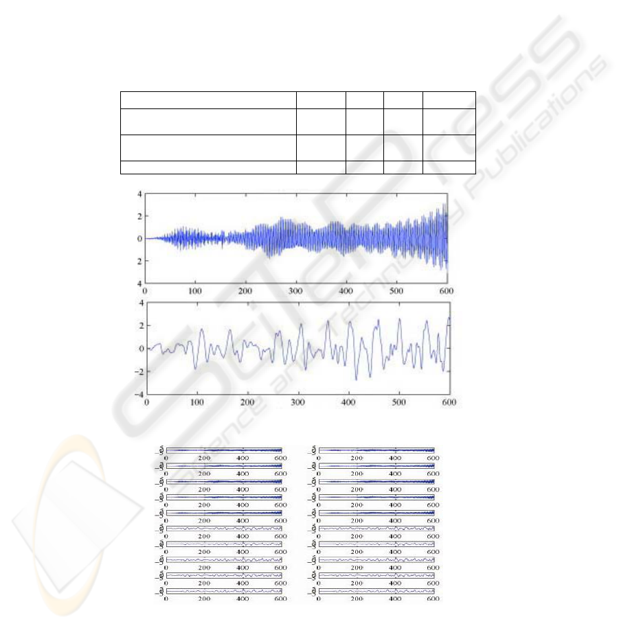
The results of a test on a two-class problem in signal recognition are presented in
Fig. 1, Fig. 2, and Fig. 3. The samples are extracted from the signals depicted in Fig.
1. In Fig. 2 are represented the initial samples. The correct recognition of 20 new
examples coming from these two classes using P1 failed in 2 cases. The correctly
recognized examples are presented in Fig. 3. The performance was improved
significantly when the volume of the initial samples increases. Using the leaving-one-
out method, the values of the resulted empirical mean error are less than 0.05 (more
than 95% new examples are correctly recognized). In order to apply the leaving-one-
out method, some first order approximations for the covariance matrices, eigen values
and eigen vectors had to be derived. The recursive equations based on first order
approximations allow to avoid the re-computing of covariance matrices, eigen vectors
and eigen values. The computations are provided in the appendix.
A series of tests were performed on P2 and they pointed out that in spite of its
higher complexity as compare to k-means, significantly increased accuracy is
obtained.
66

For instance, in case of 5 classes of data of dimensionality 6, using the first 2
principal directions, the results obtained in the compressed space are presented in Fig.
4. The examples were generated by sampling from the normal distributions for each
class. The matrix having as entries the Mahalanobis distances between classes is,
⎟
⎟
⎟
⎟
⎟
⎟
⎠
⎞
⎜
⎜
⎜
⎜
⎜
⎜
⎝
⎛
0 2.2807 1.9008 2.0341 2.8579
2.2807 0 1.7881 4.1304 2.5378
1.9008 1.7881 0 0.6417 1.5008
2.0341 4.1304 0.6417 0 3.3655
2.8579 2.5378 1.5008 3.3655 0
*10
3
.
Table 1.
The sample
ℵ
1
ℵ
2
ℵ
3
ℵ
4
Number of misclassified examples
by our method
0 0 1 0
Number of misclassified examples
by k-means
1 0 280 3
Number of iterations 2 2 3 2
Fig. 1.
Fig. 2.
67

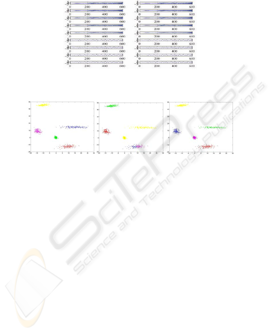
Fig. 3.
The results in case of the sample
ℵ
3
are shown in Figures 4a, 4b, and 4c.
Fig. 4a. The actual
classification.
Fig. 4b. The clusters resulted
by applying k-means.
Fig. 4c. The clusters resulted
by applying the proposed
method.
References
1. Chatterjee, C., Roychowdhury, V.P., Chong, E.K.P.: On Relative Convergence Properties
of PCA Algorithms, IEEE Trans. on Neural Networks, vol.9,no.2 (1998).
2. Cocianu, C., State, L., Rosca, I., Vlamos, P: A New Adaptive Classification Scheme Based
on Skeleton Information, Proceedings of SIGMAP 2007 (2007).
3. Diamantaras, K.I., Kung, S.Y.: Principal Component Neural Networks: theory and
applications, John Wiley &Sons, (1996).
4. Goldberger, J., Roweis, S., Hinton, G., Salakhutdinov, R.: Neighbourhood Component
Analysis, Proceedings of the Conference on Advances in Neural Information Processing
Systems (2004).
5. Gordon, A.D.: Classification, Chapman&Hall/CRC, 2
nd
Edition (1999).
6. Haykin, S., Neural Networks A Comprehensive Foundation, Prentice Hall,Inc. (1999).
7. Hastie, T., Tibshirani, R., Friedman,J.: The Elements of Statistical Learning Data Mining,
Inference, and Prediction, Springer (2001).
8. Hyvarinen, A., Karhunen, J., Oja, E. Independent Component Analysis, John Wiley &Sons
(2001).
9. Larose, D.T. Data Mining. Methods and Models, Wiley-Interscience, A John Wiley and
Sons, Inc Publication, Hoboken, New Jersey (2006).
10. Liu, J., and Chen, S. Discriminant common vectors versus neighborhood components
analysis and Laplacianfaces: A comparative study in small sample size problem. Image and
Vision Computing 24 (2006).
68

11. State, L., Cocianu, C., Vlamos, P, Stefanescu, V. PCA-Based Data Mining Probabilistic
and Fuzzy Approaches with Applications in Pattern Recognition, Proceedings of ICSOFT
2006 (2006).
12. State, L., Cocianu, C., Rosca, I., Vlamos, P: A New Learning Algorithm for Classification
in the Reduced Space, Proceedings of ICEIS 2008 (2008).
Appendix
Lemma. Let
K
XXX ,...,,
21
be an n-dimensional Bernoullian sample. We denote by
,
1
ˆ
1
∑
=
=
N
i
iN
N
Xμ
()()
∑
=
−−
−
=
N
i
T
NiNiN
N
1
ˆˆ
1
1
ˆ
μXμXΣ , and let
{
}
ni
N
i
≤≤1
λ be the eigen
values and
{
}
ni
N
i
≤≤1
ψ a set of orthogonal unit eigen vectors of
N
Σ
ˆ
, 12 −≤
≤
KN . In
case the eigen values of
1
ˆ
+N
Σ are pair wise distinct, the following first order
approximations hold,
(
)
1
1
11 +
+
++
Δ+=
N
iN
T
N
i
N
i
N
i
ψΣψ λλ
(8)
(
)
∑
≠
=
+
++
+
+
+
+
−
Δ
+=
n
ij
j
N
j
N
j
N
i
N
iN
T
N
j
N
i
N
i
1
1
11
1
1
1
1
ψ
ψΣψ
ψψ
λλ
(9)
where
11
ˆˆ
++
−=Δ
NNN
ΣΣΣ .
Proof Using the perturbation theory, we get,
11
ˆˆ
++
Δ+=
NNN
ΣΣΣ and,
11 ++
Δ+=
N
i
N
i
N
i
ψψψ
,
11 ++
Δ+=
N
i
N
i
N
i
λλλ
, ni
≤
≤
1 . Then,
()()
()()
T
NNNNNN
NN
N
N
μXμXΣΣ −−
+−
−
−
=Δ
++++ 1111
11
ˆ
1
1
(10)
where
(
)
N
N
N
NN
N
11
1
++
−
+
=
Xμ
μ
(
)
(
)
=Δ+Δ+
++
++
11
11
ˆ
N
i
N
iNN
ψψΣΣ
(
)
(
)
1111 ++++
Δ+Δ+
N
i
N
i
N
i
N
i
ψψ λλ
(11)
Using first order approximations, from (11) we get,
111111
1
1
1
1
11
ˆ
++++++
+
+
+
+
++
Δ+Δ+≅
≅Δ+Δ+
N
i
N
i
N
i
N
i
N
i
N
i
N
iN
N
iN
N
i
N
i
ψψψ
ψΣψΣψ
λλλ
λ
(12)
hence,
()
(
)
≅Δ+Δ
+
+
++
+
+ 1
1
11
1
1
ˆ
N
iN
T
N
i
N
iN
T
N
i
ψΣψψΣψ
()
2
11111 +++++
Δ+Δ≅
N
i
N
i
N
i
T
N
i
N
i
ψψψ λλ
(13)
Using
(
)( )
1
111
ˆ
+
+++
=
N
T
N
i
T
N
i
N
i
Σψψ λ we obtain ,
() ()
(
)
11111
1
1111 +++++
+
++++
Δ+Δ≅Δ+Δ
N
i
N
i
T
N
i
N
i
N
iN
T
N
i
N
i
T
N
i
N
i
λλλ ψψψΣψψψ
(14)
69

hence
()
1
1
11 +
+
++
Δ=Δ
N
iN
T
N
i
N
i
ψΣψ λ that is,
(
)
1
1
11 +
+
++
Δ+=
N
iN
T
N
i
N
i
N
i
ψΣψ λλ
(15)
The first order approximations of the orthonormal eigen vectors of
N
Σ
ˆ
can be
derived using the expansion of each vector
1+
Δ
N
i
ψ in the basis represented by the
orthonormal eigen vectors of
1
ˆ
+N
Σ ,
∑
=
++
=Δ
n
j
N
jji
N
i
b
1
1
,
1
ψψ
(16)
where
(
)
11
,
++
Δ=
N
i
T
N
jji
b ψψ
(17)
Using the orthonormality, we get,
(
)
(
)
=Δ+≅Δ+=
+++++ 11
2
1
2
11
21
N
i
T
N
i
N
i
N
i
N
i
ψψψψψ
(
)
(
)
11
21
++
Δ+=
N
i
T
N
i
ψψ
(18)
that is
(
)
11
,
++
Δ=
N
i
T
N
iii
b ψψ =0
(19)
Using (11), the approximation,
11111
1
1
1
ˆ
+++++
+
+
+
Δ+Δ≅Δ+Δ
N
i
N
i
N
i
N
i
N
iN
N
iN
ψψψΣψΣ λλ
(20)
holds for each
ni ≤≤1 .
For
nij ≤
≠
≤1 , from (20) we obtain the following equations,
()
(
)
≅Δ+Δ
+
+
++
+
+ 1
1
11
1
1
ˆ
N
iN
T
N
j
N
iN
T
N
j
ψΣψψΣψ
()
(
)
111111 ++++++
Δ+Δ≅
N
i
T
N
j
N
i
N
i
T
N
j
N
i
ψψψψ λλ
(21)
() ()
(
)
1111
1
11
1
1
ˆ
++++
+
++
+
+
Δ≅Δ+Δ
N
i
T
N
j
N
i
N
iN
T
N
j
N
iN
T
N
j
ψψψΣψψΣψ λ
(22)
()
(
)
(
)
1111
1
1111 ++++
+
++++
Δ≅Δ+Δ
N
i
T
N
j
N
i
N
iN
T
N
j
N
i
T
N
j
N
j
ψψψΣψψψ λλ
(23)
From (23) we get,
()
(
)
11
1
1
1
11
,
++
+
+
+
++
−
Δ
=Δ=
N
j
N
i
N
iN
T
N
j
N
i
T
N
jji
b
λλ
ψΣψ
ψψ
(24)
Consequently, the first order approximation of the eigen vectors of
N
Σ
ˆ
are,
(
)
∑
≠
=
+
++
+
+
+
+++
−
Δ
+≅Δ+
n
ij
j
N
j
N
j
N
i
N
iN
T
N
j
N
i
N
i
N
i
1
1
11
1
1
1
111
ψ
ψΣψ
ψψψ
λλ
(25)
70