
ABOUT THE DECOMPOSITION OF RATIONAL SERIES IN
NONCOMMUTATIVE VARIABLES INTO SIMPLE SERIES
Mikhail V. Foursov
IRISA/Universit´e de Rennes–1, Campus Universitaire de Beaulieu, 35042 Rennes Cedex, France
Christiane Hespel
IRISA/INSA de Rennes, 20, avenue des Buttes de Co¨esmes, 35043 Rennes Cedex, France
Keywords:
Formal power series, Generating series, Rational series, Joint matrix block–diagonalization, Dynamical sys-
tems.
Abstract:
Similarly to the partial fraction decomposition of rational fractions, we provide an approach to the decom-
position of rational series in noncommutative variables into simpler series. This decomposition consists in
splitting the representation of the rational series into simpler representations. Finally, the problem appears as
a joint block–diagonalization of several matrices. We present then an application of this decomposition to the
integration of dynamical systems.
1 INTRODUCTION
This article deals with the problem of splitting a ratio-
nal formal power series into simple series. We present
first well–known results on decomposition of rational
series in a single variable and on reduced linear repre-
sentations of a rational series in noncommutativevari-
ables.
Fliess showed that decomposition of rational
formal power series can be done by joint block-
diagonalization of several matrices. This is a diffi-
cult problem which was approached by numerous re-
searchers such as Gantmacher, Jordan, Dunford and
Jacobi.
The decomposition into simple series has many
different applications in the dynamical system theory
(such as subsystem independence, integration or sta-
bility) and in the automata theory, among others. We
illustrate the application to the integration of dynami-
cal systems.
2 PRELIMINARIES
In this paper, we consider a rational series s with co-
efficients in the field K = C. In some sections, K can
be taken as a semi–ring or as a commutative field.
2.1 Decomposition of Rational Series in
a Single Variable into Simple Series
A rational series s in a single variable can be rewritten
as a rational fraction (Gantmacher, 1966).
Theorem 2.1. Let s =
∑
∞
j=0
s
j
X
j+1
∈ K[[X]] be a for-
mal power series with coefficients in a field K of char-
acteristic 0. Then there are 2 polynomials P,Q ∈
K[X], such that
deg(Q) < deg(P),
Q
P
=
∞
∑
j=0
s
j
X
j+1
(1)
if and only if there is an integer p ∈ N such that the
ranks of the Hankel matrices of orders k, ∀k ≥ p, are
all equal to p.
In this case there exist polynomials P of degree p
and Q of degree at most p − 1. The minimal possi-
ble degree of P is p, and the pair (P, Q) is completely
determined by these degree conditions and the condi-
tion that P is monic. The polynomials P and Q are
then prime.
The proof of this theorem is based on the resolu-
tion of a system of linear equations obtained by iden-
tifying the coefficients of X
l
. Let us remark that the
finiteness condition on the rank of the Hankel matrix
of s expresses the recognizability of s, that is the ra-
tionality, for a single variable. This rational fraction
can be easily split up into simple fractions of the form
214
V. Foursov M. and Hespel C. (2009).
ABOUT THE DECOMPOSITION OF RATIONAL SERIES IN NONCOMMUTATIVE VARIABLES INTO SIMPLE SERIES.
In Proceedings of the 6th International Conference on Informatics in Control, Automation and Robotics - Signal Processing, Systems Modeling and
Control, pages 214-220
DOI: 10.5220/0002197602140220
Copyright
c
SciTePress

s
i
=
a
i
(1−α
i
X)
r
i
where a
i
,α
i
∈ C,r
i
∈ N, s
i
being ex-
panded as a rational simple series.
Remark. A rational series can be considered as a
weighted automaton (also known as automaton with
multiplicity). The previous decomposition of s as
s =
∑
i∈I
s
i
appears as a decompositionof the weighted
automaton A
s
of dimension r into ∪
i∈I
A
s
i
, where A
s
i
are simple independent automata of dimension r
i
such
that
dim(A
s
i
) = r
i
∑
i∈I
r
i
= r
(2)
2.2 Reduced Linear Representation of
Rational Series in Noncommutative
Variables
2.2.1 Series in Noncommutative Variables
These definitions and notations are from (Berstel and
Reutenauer, 1988; Reutenauer, 1980; Salomaa and
Soittola, 1978; Sch¨utzenberger, 1961). K is a semi–
ring.
Definition 2.1. (Formal power series in noncommu-
tative variables)
1. An alphabet X is a nonempty finite set. Elements
of X are letters. The free monoid X
∗
generated by
the alphabet X is the set of finite words X
i
1
··· X
i
l
,
where X
i
j
∈ X, including the empty word denoted
by 1. The set X
∗
is a monoid with respect to con-
catenation.
2. A formal power series s in noncommutative vari-
ables is a function
s : X
∗
→ K (3)
The coefficient s(w) of the word w in the series s
is denoted by hs|wi.
3. The set of formal power series s over X with co-
efficients in K is denoted by KhhXii. A structure
of semi–ring is defined on KhhXii by the sum and
the Cauchy product. Two external operations (left
and right products) from K to KhhXii are also de-
fined. The set of polynomials is denoted by KhXi.
2.2.2 Rational Series in Noncommutative
Variables
Definition 2.2. (Rational formal power series in non-
commutative variables)
1. The rational operations in KhhXii are the sum,
the product, two external products as well as the
Kleene star operation defined by T
∗
=
∑
n≥0
T
n
for a proper series T (i.e. such that hT|1i = 0).
2. A subset of KhhXii is rationally closed if it is
closed under the rational operations. The small-
est rationally–closed subset containing a subset
E ⊆ KhhXii is called the rational closure of E.
3. A series s is rational if s is an element of the ra-
tional closure of KhXi.
2.2.3 Recognizable Series in Noncommutative
Variables
We propose several equivalent definitions (Berstel
and Reutenauer, 1988; Fliess, 1977; Fliess, 1974;
Fliess, 1976; Jacob, 1980), K being a commutative
field.
Definition 2.3. (Recognizable formal power series in
noncommutative variables)
1. A series s ∈ KhhXii is recognizable if there exists
an integer N ≥ 1, a monoid morphism
µ : X
∗
→ K
N∗N
(4)
and 2 matrices λ ∈ K
1∗N
and γ ∈ K
N∗1
such that
∀w ∈ X
∗
, hs|wi = λµ(w)γ. (5)
2. A series s ∈ KhhXii is recognizable if there ex-
ists an integer N, the rank of its Hankel matrix
H(s) = (hs|w
1
.w
2
i)
w
1
,w
2
∈X
∗
. The first row of H(s)
indexed by the word 1 describes s. The other rows
are the remainders of s by a word w. For instance,
the row L
X
1
represents the right remainder of s by
X
1
, denoted by s⊲ X
1
.
3. A series s ∈ KhhXii is recognizable if it is de-
scribed by a finite weighted automaton obtained
from its Hankel matrix remainders.
Definition 2.4. The triple (λ,µ,γ) is called a linear
representation of s. The representation with minimal
dimension is called the reduced linear representation.
2.2.4 Theorem of Sch¨utzenberger
For a series in several noncommutative variables, the
theorem of Sch¨utzenbergerproves the equivalence be-
tween the notions of rationality and of recognizabil-
ity (Sch¨utzenberger, 1961; Berstel and Reutenauer,
1988).
Theorem 2.2. A formal series is recognizable if and
only if it is rational.
2.2.5 Finite Weighted Automaton Obtained
from a Rational Series
This method is developed in (Hespel, 1998). It is
based on the following theorem (Fliess, 1976; Jacob,
1980).
ABOUT THE DECOMPOSITION OF RATIONAL SERIES IN NONCOMMUTATIVE VARIABLES INTO SIMPLE
SERIES
215

Theorem 2.3. A formal series s ∈ RhhXii is recog-
nizable if and only if its rank N is finite. Then it is
recognized by a R–matrix automaton M = (N,γ,λ,µ).
Two sets of words {g
i
}
1≤i≤N
and {d
j
}
1≤ j≤N
, whose
lengths are < N, can be determined so that the appli-
cation χ from X
∗
to R
N×N
defined by
(χ(w))
i, j
= hs|g
i
.w.d
j
i (6)
satisfies χ(w) = χ(1)µ(w) with χ(1) invertible.
1. The method consists in extracting from the Han-
kel matrix H(s) (whose rank is N) a system B of
N row vectors (L
w
i
)
i∈I
(resp. N column vectors
(C
w
j
)
j∈J
), indexed by some words of minimum
length, such that their determinant is nonzero and
such that every row (resp. every column) of H(s)
can be expressed as a linear combination of el-
ements of B. These relations allow us to define
∀X
k
∈ X the matrices µ(X
k
) describing the action
of the letter X
k
on the row vector L
w
i
(resp. the
column vector C
w
j
). The first row (resp. the first
column) of B defines λ. γ is the initial vector
(1 0··· 0)
T
. The series s can thus be written
s =
∑
w∈X
∗
hs|wi =
∑
w∈X
∗
λµ(w)γ (7)
2. We define, based on the basis B and matrices
µ(X
i
), γ and λ, a finite weighted (left or right) au-
tomaton A = {X,Q,I,A, τ} such that
• X is the alphabet,
• the state set is Q = {L
w
i
}
i∈I
representing {s ⊲
w
i
}
i∈I
(resp. Q = {C
w
j
}
j∈J
representing {w
j
⊳
s}
j∈J
),
• the first row (resp. the first column) I of B is the
initial state,
• every transition between states belonging to τ
is labeled by a letter X
i
∈ X and labeled by the
coefficient appearing in the linear dependence
relation,
• A is the final state set; it is the set of rows L
w
(resp. the columnsC
w
) of B such that hs|wi 6= 0.
3 DECOMPOSITION OF
RATIONAL SERIES :
PRINCIPLE
3.1 Theoretical Results
In his thesis (Fliess, 1977), M.Fliess gives the idea of
a unique decomposition of the reduced matrix repre-
sentation µ associated to a rational series s into the di-
rect sum of a finite number of simple representations.
His idea is based on the Krull–Schmidt theorem.
Let us recall some definitions and notations (Bers-
tel and Reutenauer, 1988; Fliess, 1977).
Let s ∈ KhhXii be a rational series. Let us denote
by {N,λ,µ(X
∗
),γ}, or rather by µ, its reduced matrix
representation. The coefficients of s satisfy
hs|wi = λµ(w)γ, ∀w ∈ X
∗
(8)
For a decomposition of µ
µ = ⊕
k
i=1
µ
i
(9)
the associated decompositions of the vectors λ and γ
are
λ = ⊕
k
i=1
λ
i
, γ = ⊕
k
i=1
γ
i
(10)
The series s is then split up into s =
∑
k
i=1
s
i
, where
every rational series satisfies
s
i
=
∑
w∈X
∗
λ
i
µ
i
(w)γ
i
w (11)
Among {s
i
}
1≤i≤k
there can exist a subfamily with
indices J ⊆ {1,· · · ,k} such that ∀ j ∈ J, the represen-
tation µ
j
is nilpotent.
• A representation µ
i
is nilpotent if and only if
∀w ∈ X
+
, µ
j
(w) is nilpotent.
Using Levitzki theorem (Kaplanski, 1969), the
semi–group of nilpotent matrices {⊕
j∈J
µ
j
(w), w ∈
X
+
} is simultaneously triangulable. Particularly, for
every word w of sufficient length, ⊕
j∈J
µ
j
(w) is the
zero matrix. Then the sum
∑
j∈J
s
j
of the series as-
sociated to this decomposition into nilpotent matrices
is a polynomial representing the polynomial part of s.
Let us consider now the representations which
cannot be decomposed and which are not nilpotent.
• Such a representation µ
i
is associated with a sim-
ple series s
i
.
• Two series s
1
and s
2
are called relatively prime if
and only if
∀α, β ∈ C\{0},
rank(αs
1
+ βs
2
) = rank(s
1
) + rank(s
2
)
(12)
We can express the following theorem (Fliess,
1977)
Theorem 3.1. K being a field, there is a unique way
for decomposing every rational series s∈ KhhXii into
the sum of its polynomial part and of some simple ra-
tional relatively prime series.
ICINCO 2009 - 6th International Conference on Informatics in Control, Automation and Robotics
216

3.2 Approaches of the Simultaneous
Decomposition of Matrices {A
i
}
i∈I
We restrict the number of matrices to two in order
to simplify the explanations. The problem is the fol-
lowing : to provide a simultaneous decomposition of
A
1
and A
2
into a nilpotent part A
1
n
,A
2
n
and a block–
diagonalizable part A
1
d
,A
2
d
, in some basis.
This problem is difficult. We present some ap-
proaches from Gantmacher, Jordan, Dunford and Ja-
cobi.
1. First Approach : Gantmacher
Gantmacher considers the linear pencil A
1
+ λA
2
of the matrices A
1
,A
2
. By using elementary trans-
formations, ((Gantmacher, 1966), tome 1, Chap-
ter 2), the original regular/singular pencil can
be reduced to a quasi–diagonal canonical form
((Gantmacher, 1966), tome 2, Chapter 12). The
original pencil A
1
+ λA
2
and the canonical pen-
cil A
′
1
+ λA
′
2
are then equivalent but generally not
similar : there exist some regular matrices P,Q
such that A
′
1
+ λA
′
2
= P(A
1
+ λA
2
)Q but generally
Q 6= P
−1
.
2. Second Approach : Jordan, Dunford
These methods are suitable for a single matrix.
The Jordan’s method consists in computing 2 reg-
ular matrices P,Q and irreducible block diagonal
matrices A
′
1
,A
′
2
such that
A
1
= P
−1
A
′
1
P, A
2
= Q
−1
A
′
2
Q. (13)
So one can use the Jordan decomposition A
′
1
and A
′
2
of each matrix in order to initialize a si-
multaneous decomposition in block diagonal ma-
trices of suitable size. The knowledge of the
eigenspaces (E
1
i
) and (E
2
i
) of A
1
and A
2
allows
to set some bounds on the size of the blocks.
The Dunford decomposition into a diagonalizable
part and a nilpotent part can be provided from the
Jordan decomposition.
3. Approach by Jacobi Algorithms
When the sizes of the decomposition blocks are
known, the method consists in providing a joint
block–diagonalizer. This matrix is iteratively
computed as a product of Givens rotations. The
convergence of this algorithm is proven but not
necessary to obtain an optimal solution.
4 DECOMPOSITION OF
RATIONAL SERIES IN
PRACTICE
Theorem 4.1. A rational series can be decomposed
into a sum of simpler series using matrix joint block–
decomposition.
Proof. Let s be a rational series s =
∑
w∈X
∗
hs|wi =
∑
w∈X
∗
λµ(w)γ. For a simultaneous change of basis
matrix P for µ(x
i
j
)
i
j
, we have
hs|x
i
1
··· x
i
l
i = λµ(x
i
1
)··· µ(x
i
l
)γ =
= λPµ
′
(x
i
1
)P
−1
··· Pµ
′
(x
i
l
)P
−1
γ
= (λP)µ
′
(x
i
1
)··· µ
′
(x
i
l
)(P
−1
γ) =
= λ
P
µ
P
(x
i
1
)··· µ
P
(x
i
l
)γ
P
(14)
Thus, when µ
′
(x
i
1
),··· ,µ
′
(x
i
l
) are decomposed into
block–diagonal matrices, we obtain the decomposi-
tion of s into corresponding simpler series.
Example 1. A representation of the series is given
by the finite weighted automaton
1 2
x
2
x
2
x
1
x
1
The actions of the letters x
1
and x
2
are given by the
matrices
µ(x
1
) =
1 0
0 1
and µ(x
2
) =
0 1
1 0
(15)
The initial vector is
γ =
1
0
(16)
and the covector is
λ =
0 1
. (17)
The eigenvalues of µ(x
2
) are λ
1
= 1 and λ
2
= −1. In
the basis B of the eigenvectors, the matrices µ(x
1
) and
µ(x
2
) are
µ(x
1
)
P
=
1 0
0 1
and µ(x
2
)
P
=
1 0
0 −1
(18)
The initial vector is now
γ
P
=
1/2
1/2
(19)
and the covector is
λ
P
=
1 −1
. (20)
ABOUT THE DECOMPOSITION OF RATIONAL SERIES IN NONCOMMUTATIVE VARIABLES INTO SIMPLE
SERIES
217

Thus this series can be decomposed into series s
1
and
s
2
: s = s
1
+ s
2
. The representation of s
1
is
µ
1
(x
1
) = (1), µ
1
(x
2
) = (1), γ
1
= (1/2), λ
1
= (1).
(21)
For s
2
we have
µ
2
(x
1
) = (1), µ
2
(x
2
) = (−1), γ
1
= (1/2), λ
1
= (−1).
(22)
Example 2. Now let us consider the series with
the following representation. The actions of theletters
x
1
and x
2
are given by the matrices
µ(x
1
) =
0 0
1 1
and µ(x
2
) =
1 1
0 0
(23)
The initial vector is
γ =
1
0
(24)
and the covector is
λ =
0 1
(25)
There is no decomposition of s.
Example 3. Finally, let us consider the series
whose Hankel matrix is shown in Table 1.
The rank of this Hankel matrix is 6. We se-
lect the independent rows {L
1
,L
x
1
,L
x
2
,L
x
1
x
2
,L
x
2
x
1
x
2
,
L
x
1
x
2
x
1
x
2
} and the columns associated with the same
words. This determinant has a maximal rank = 6.
The matrices µ(x
1
) et µ(x
2
) describe the action of
the letters x
1
and x
2
.
µ(x
1
) =
0 0 0 0 0 0
1 0 0 0 0 0
0 1 1 0 1 0
0 0 0 0 0 0
0 0 0 1 0 1
0 0 0 0 0 0
(26)
and
µ(x
2
) =
0 0 0 0 0 0
0 0 0 0 0 0
1 0 1 1 0 1
0 1 0 0 0 0
0 0 0 0 0 0
0 0 0 0 1 0
(27)
The initial vector is
γ =
1 0 0 0 0 0
T
(28)
and the covector is
λ =
3 1 1 3 1 2
. (29)
By using the Jordan reduction on µ(x
1
) (with Maple)
we obtain
A = µ(x
1
)
P
=
0 1 0 0 0 0
0 0 0 0 0 0
0 0 1 0 0 0
0 0 0 0 1 0
0 0 0 0 0 0
0 0 0 0 0 0
(30)
where the change of basis matrix is
P =
0 0 0 0 −1 0
0 0 0 −1 0 0
−1 −1 1 0 0 0
0 0 0 0 0 −1
1 0 0 1 0 0
0 1 0 0 1 1
(31)
By this change of basis, µ(x
2
) becomes
B = µ(x
2
)
P
=
0 0 0 0 0 0
1 0 0 0 0 0
0 0 1 0 0 0
0 0 0 0 0 0
0 0 0 0 0 0
0 0 0 1 0 0
(32)
In this new basis
λ
P
=
0 1 1 0 −1 −1
(33)
and
γ
P
=
0 1 1 0 −1 0
T
(34)
In this case, we are lucky and the matrices A and B
corresponding to µ(x
1
)
P
and µ(x
2
)
P
in the same basis
directly present 3 diagonal blocks :
• the upper left block of size 2 corresponding to the
series s
1
=
1
1− x
1
x
2
,
• the middle block of size 1 corresponding to the
series s
2
=
1
1− (x
1
+ x
2
)
,
• the lower right block of size 3 corresponding to
the polynomial s
3
= 1 + x
1
x
2
. This last block is
associated to a nilpotent representation.
5 AN APPLICATION TO
DYNAMICAL SYSTEMS
Definition 5.1. A bilinear dynamical system is a sys-
tem of ordinary differential equations of the form
˙
q(t) =
M
0
+
m
∑
i=1
u
i
(t)M
i
q(t)
s(t) =λ · q(t),
(35)
where
ICINCO 2009 - 6th International Conference on Informatics in Control, Automation and Robotics
218
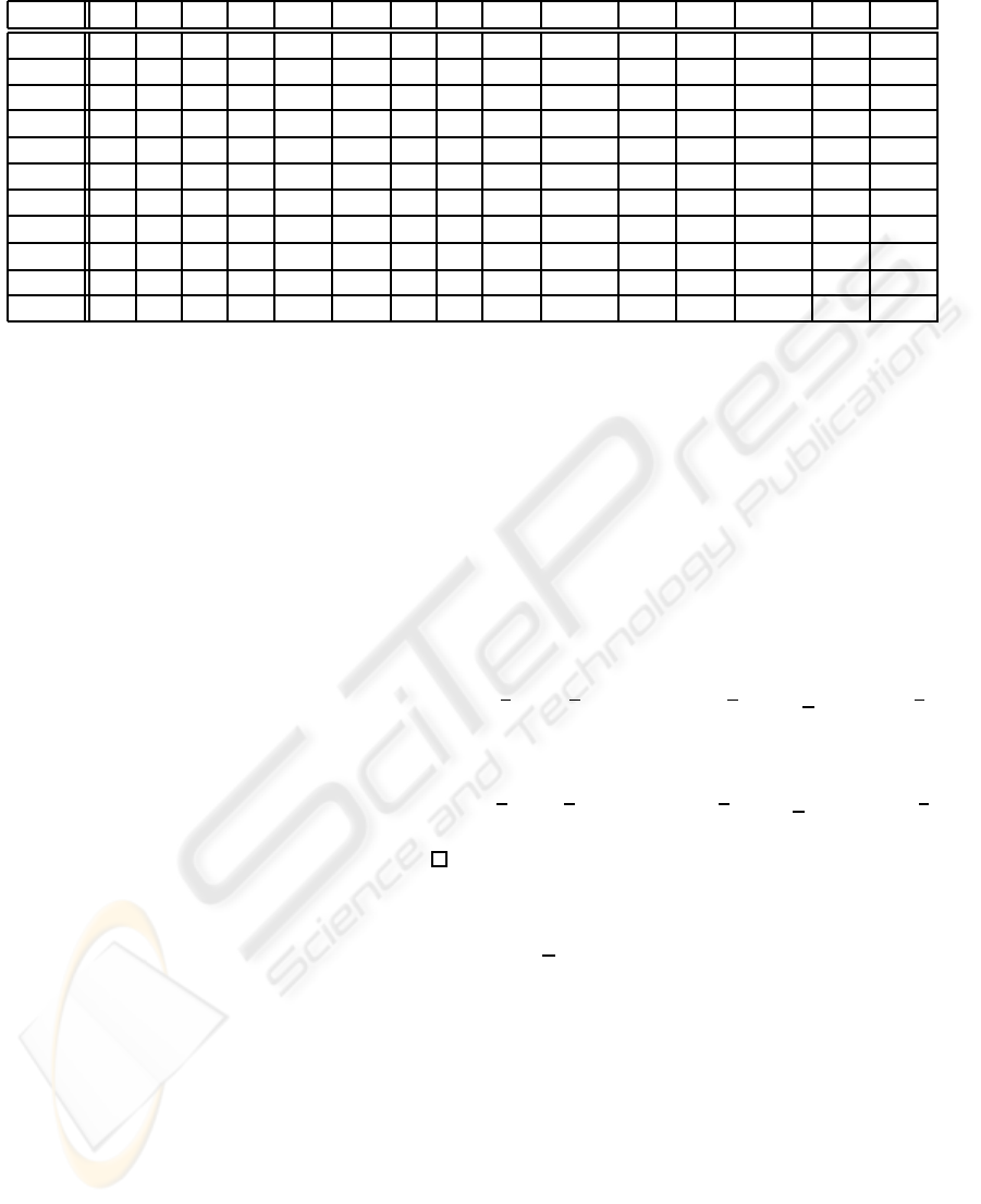
Table 1: Hankel matrix of example 3.
1 x
1
x
2
x
2
1
x
1
x
2
x
2
x
1
x
2
2
x
3
1
x
2
1
x
2
x
1
x
2
x
1
x
1
x
2
2
x
2
x
2
1
x
2
x
1
x
2
x
2
2
x
1
x
3
2
···
1 3 1 1 1 3 1 1 1 1 1 1 1 1 1 1·· ·
x
1
1 1 3 1 1 1 1 1 1 1 1 1 2 1 1·· ·
x
2
1 1 1 1 1 1 1 1 1 1 1 1 1 1 1·· ·
x
2
1
1 1 1 1 1 1 1 1 1 1 1 1 1 1 1·· ·
x
1
x
2
3 1 1 1 2 1 1 1 1 1 1 1 1 1 1·· ·
x
2
x
1
1 1 1 1 1 1 1 1 1 1 1 1 1 1 1·· ·
x
2
2
1 1 1 1 1 1 1 1 1 1 1 1 1 1 1·· ·
x
3
1
1 1 1 1 1 1 1 1 1 1 1 1 1 1 1·· ·
x
2
1
x
2
1 1 1 1 1 1 1 1 1 1 1 1 1 1 1·· ·
x
1
x
2
x
1
1 1 2 1 1 1 1 1 1 1 1 1 2 1 1·· ·
··· ··· ··· ·· · ··· ·· · ·· · ··· ··· ·· · ·· · ··· · ·· ··· ·· · ···
1. u(t) = (u
1
(t), . .., u
n
(t)) ∈ R
n
is the (partwise
continuous) input vector,
2. q(t) ∈ M is the current state, where M is a real
differential manifold, usually R
m
,
3. s(t) ∈ R is the output function.
Definition 5.2. The generating series G of a bilinear
dynamical system (Fliess, 1981) is a formal power se-
ries with the alphabet X = {z
o
,z
1
,... z
m
}, where z
i
for
j > 0 correspond to the input u
i
(t) whereas z
0
corre-
sponds to the drift. It is defined by
hG|z
j
0
··· z
j
k
i = λ· M
j
0
···M
j
k
· q(0). (36)
Theorem 5.1. The generating series of bilinear dy-
namical system are rational. Inversely, every rational
series is a generating series of a bilinear dynamical
system.
Proof. We take µ such that µ(z
i
) = M
i
for i ≥ 0 and
we denote γ = q(0). It follows directly that hλ,µ,γi is
a rational series.
Definition 5.3. The Chen series measures the input
contribution (Chen, 1971), and is independent of the
system. The coefficients of the Chen series are cal-
culated recursively by integration using the following
two relations :
• hC
u
(t)|1i = 1,
• hC
u
(t)|wi =
Z
t
0
hC
u
(τ)|viu
j
(τ)dτ for a word w =
z
j
v.
The causal functional y(t) is then obtained locally
as the product of the generating series and the Chen
series :
y(t) = hG||C
u
(t)i =
∑
w∈X
∗
hG|wihC
u
(t)|wi (37)
This formula is known as the Peano–Baker formula,
as well as the Fliess’ fundamental formula.
Now we apply the decomposition in the 3 above
examples to the corresponding dynamical systems
(identifying z
0
with x
1
and z
1
with x
2
).
Example 1. The correspondingdynamical system
is
y
′
1
(t) = y
1
(t) + u(t)y
2
(t), y
1
(0) = 1,
y
′
2
(t) = y
2
(t) + u(t)y
1
(t), y
2
(0) = 0,
s(t) = y
2
(t).
(38)
Maple gives its solution is some complicated form.
However using our decompositioninto two dynamical
systems
y
′
1
(t) = y
1
(t)(1+ u(t)), y
1
(0) =
1
2
, s
1
(t) = y
1
(t)
(39)
and
y
′
2
(t) = y
2
(t)(1−u(t)), y
2
(0) =
1
2
, s
2
(t) = −y
2
(t)
(40)
we can easily obtain that
s(t) = s
1
(t) + s
2
(t) =
=
1
2
exp
Z
t
0
(1+ u(τ))dτ) − exp
Z
t
0
(1− u(τ))dτ
(41)
Example 2. The correspondingdynamical system
is
y
′
1
(t) = u(t)(y
1
(t) + y
2
(t)), y
1
(0) = 1,
y
′
2
(t) = y
1
(t) + y
2
(t), y
2
(0) = 0,
s(t) = y
2
(t).
(42)
We can compute its solution directly
s(t) =
Z
t
0
exp
Z
τ
1
0
(1+ u(τ
2
)dτ
2
dτ
1
. (43)
s(t) cannot be decomposed as a sum of two simpler
expressions.
ABOUT THE DECOMPOSITION OF RATIONAL SERIES IN NONCOMMUTATIVE VARIABLES INTO SIMPLE
SERIES
219

Example 3. The correspondingdynamical system
cannot be solved directly. However, using the above
decomposition we obtain s(t) = s
1
(t) + s
2
(t) + s
3
(t),
where
s
1
(t) =1+
Z
t
0
Z
τ
1
0
u(τ
2
)dτ
2
dτ
1
+
Z
t
0
Z
τ
1
0
u(τ
2
)
Z
τ
2
0
Z
τ
3
0
u(τ
4
)dτ
4
dτ
3
dτ
2
dτ
1
+ · · ·
(44)
corresponds to the first dynamical system and is the
solution of the system
y
′
1
(t) = s
2
(t), y
1
(0) = 0,
y
′
2
(t) = u(t)s
1
(t), y
2
(0) = 1,
s
1
(t) = y
2
(t).
(45)
whereas
s
2
(t) = exp
Z
t
0
(1+ u(τ))dτ
(46)
corresponds to the second dynamical system and
s
3
(t) = 1+
Z
t
0
Z
τ
1
0
u(τ
2
)dτ
2
dτ
1
(47)
is the solution of the third system.
6 CONCLUSIONS
In this paper, we presented an approach to the prob-
lem of decomposition of rational series in noncom-
mutative variables into some simple series. The study
of the simultaneous block–diagonalization has yet to
be improved. We present an application of this de-
composition to dynamical systems.
There are numerous further applications of this
decomposition to dynamical systems and automata :
• The study of the stability of bilinear systems can
be approachedby using its generating series (Ben-
makrouha and Hespel, 2007) : in some cases, the
output can be explicitly computed or bounded.
The decomposition of this series into simple se-
ries would simplify this study in the other cases.
• In a bilinear system, the dependence or the inde-
pendenceof subsystems can be studied via the de-
composition of the generating series of the sys-
tem.
• A finite weighted automaton being another rep-
resentation of a rational series, the property of de-
composition of a rational series into simpler series
is transferred to the corresponding finite weighted
automaton. So we can define a simpler finite
weighted automaton.
REFERENCES
Benmakrouha F. and Hespel C. (2007). Generating formal
power series and stability of bilinear systems, 8th Hel-
lenic European Conference on Computer Mathemat-
ics and its Applications (HERCMA 2007).
Berstel J. and Reutenauer C. (1988). Rational series and
their languages, Springer–Verlag.
Chen K.-T. (1971). Algebras of iterated path integrals and
fundamental groups, Trans. Am. Math. Soc., 156,
359–379.
Fevotte C. and Theis F.J. (2007). Orthonormal approximate
joint block–diagonalization, technical report, Telecom
Paris.
Fliess M. (1972). Sur certaines familles de s´eries formelles,
Th`ese d’´etat, Universit´e de Paris–7.
Fliess M. (1974) Matrices de Hankel, J. Maths. Pur. Appl.,
53, 197-222.
Fliess M. (1976). Un outil alg´ebrique : les s´eries formelles
non commutatives, in “Mathematical System Theory”
(G. Marchesini and S.K. Mitter Eds.), Lecture Notes
Econom. Math. Syst., Springer Verlag, 131, 122-148.
Fliess M. (1981). Fonctionnelles causales non lin´eaires et
ind´etermin´ees non commutatives, Bull. Soc. Math.
France, 109, 3–40.
Gantmacher F.R. (1966). Th´eorie des matrices, Dunod.
Hespel C. (1998). Une ´etude des s´eries formelles non com-
mutatives pour l’Approximation et l’Identification des
syst`emes dynamiques, Th`ese d’´etat, Universit´e de
Lille–1.
Hespel C. and Martig C. (2006). Noncommutative comput-
ing and rational approximation of multivariate series,
Transgressive Computing 2006, 271-286.
Jacob G. (1980) R´ealisation des syst`emes r´eguliers (ou
bilin´eaires) et s´eries g´en´eratrices non commutatives,
S´eminaire d’Aussois, RCP567, Outils et mod`eles ma-
th´ematiques pour l’Automatique, l’Analyse des Sys-
t`emes, et le traitement du Signal.
Kaplanski I. (1969). Fields and rings, The University of
Chicago Press, Chicago.
Reutenauer C. (1980). S´eries formelles et alg`ebres syntac-
tiques, J. Algebra, 66, 448-483.
Salomaa A. and Soittola M. (1978). Automata Theoretic
aspects of Formal Power Series, Springer.
Sch¨utzenberger M.P (1961). On the definition of a family
of automata, Inform. and Control, 4, 245-270.
ICINCO 2009 - 6th International Conference on Informatics in Control, Automation and Robotics
220
