
ITERATIVE FEEDBACK TUNING APPROACH TO A CLASS OF
STATE FEEDBACK-CONTROLLED SERVO SYSTEMS
Mircea-Bogdan Rădac, Radu-Emil Precup
Dept. of Automation and Appl. Inf., “Politehnica” University of Timisoara
Bd. V. Parvan 2, 300223 Timisoara, Romania
Emil M. Petriu
School of Information Technology and Eng., University of Ottawa
800 King Edward, Ottawa, ON, K1N 6N5 Canada
Stefan Preitl, Claudia-Adina Dragoş
Dept. of Automation and Appl. Inf., “Politehnica” University of Timisoara
Bd. V. Parvan 2, 300223 Timisoara, Romania
Keywords: Iterative Feedback Tuning, Servo systems, State feedback control systems.
Abstract: An original control structure dedicated to a class of second-order state feedback control systems is presented
in the paper. The controlled processes are accepted to be characterized by second-order servo systems with
integral component. Optimal state feedback control systems are designed for those processes making use of
the Iterative Feedback Tuning (IFT) approach. The state feedback control system structure is extended with
an integral component to ensure the rejection of constant disturbances. A case study concerning the position
control of a DC servo system with backlash is included. Real-time experimental results validate the
theoretical part of the IFT approach.
1 INTRODUCTION
The second-order servo systems with integral
component are applied widely as controlled
processes in real-world applications including
mechatronics, electrical drives, sub-systems in
power plant control systems, positioning systems in
manipulators, mobile robots, machine tools, flight
guidance and control (Škrjanc et al., 2005; Gomes et
al., 2007; Petres et al., 2007; Barut et al., 2008;
Costas-Perez et al., 2008; Denève et al., 2008; De
Santis et al., 2008; Orlowska-Kowalska and Szabat,
2008; Precup et al., 2008b; Vaščák, 2008). Those
controlled processes are acknowledged as particular
cases of benchmark systems (Åström and Hägglund,
2000; Isermann, 2003; Horváth and Rudas, 2004;
Kovács, 2006). Accepting that they are linearized
versions of nonlinear servo systems, the parameters
are variable with respect to the operating points.
Hence the parameter variation makes their control a
challenging task when very good control system
performance indices are required. Their control
problems become even more challenging when low-
cost automation solutions are needed in the design
and implementation of the control system structures.
One control solution to cope with the accepted
class of processes described is represented by state
feedback control systems. Since the main control
aims, high performance indices in reference input
tracking and regulation with respect to several types
of load disturbance inputs, are difficult to be
fulfilled, one typical approach is to design optimal
control systems. The improvement of the control
system performance indices (fore example settling
time and overshoot) is enabled by the minimization
of appropriately defined objective functions
resulting in optimal state feedback control systems.
An alternative to the minimization of the objective
functions is represented by Iterative Feedback
Tuning (IFT) (Hjalmarsson et al., 1994, 1998). IFT
41
R
ˇ
adac M., Precup R., Petriu E., Preitl S. and Drago¸s C. (2009).
ITERATIVE FEEDBACK TUNING APPROACH TO A CLASS OF STATE FEEDBACK-CONTROLLED SERVO SYSTEMS.
In Proceedings of the 6th International Conference on Informatics in Control, Automation and Robotics - Intelligent Control Systems and Optimization,
pages 41-48
DOI: 10.5220/0002204400410048
Copyright
c
SciTePress

algorithms make use of the input-output data
measured from the closed-loop system during its
operation to calculate the estimates of the gradients
and Hessians of the objective functions. Several
experiments are done per iteration and the updated
controller parameters are calculated based on the
input-output data and the estimates.
The application of IFT to one-degree-of-freedom
controllers needs two experiments per iteration. The
first experiment is referred to as the normal one and
it corresponds to the usual operation of the control
system. The second experiment is the gradient one.
The reference input in the gradient experiment is the
control error of the first experiment. An additional
normal experiment is needed in case of two-degree-
of-freedom controllers. Even more experiments are
needed to tune the state feedback controllers and the
Multi Input-Multi Output (MIMO) ones. So it is
natural to strive for the alleviation of the number of
experiments (Hjalmarsson and Birkeland, 1998;
Hjalmarsson, 1999; Jansson and Hjalmarsson,
2004).
The paper aims three main contributions. The
first contribution of the paper is the proposal of an
IFT algorithm resulting in a method to obtain the
partial derivatives needed in the calculation of the
gradient of the objective function in state feedback
control systems. The second contribution concerns
the new experiments to be done in the IFT of the
accepted class of second-order state feedback
control systems dedicated to servo systems. The
third contribution involves the highlighting of the
specific aspects related to the actuator saturation
problem proved by the low-cost implementation and
the real-time experimental results included. The
main advantages of the contributions are the
simplification of the experiments and the smooth
decrease of the objective function. Thus the local
minimum will be reached.
The paper treats the following topics. The
controlled processes and the new IFT algorithm
dedicated to the accepted class of state feedback
control system are presented in Section 2. Next,
Section 3 points out original and attractive aspects
concerning the actuator saturation problem. A case
study concentrated on the state feedback position
control of a DC servo system with backlash is
described in Section 4. The real-time experimental
results validate the IFT algorithm. The conclusions
are drawn in Section 5.
2 CONTROLLED PROCESS AND
IFT ALGORITHM
The controlled process as part of servo systems is
characterized by the following state-space model:
⎥
⎦
⎤
⎢
⎣
⎡
ω
α
=
⎥
⎦
⎤
⎢
⎣
⎡
⎥
⎥
⎦
⎤
⎢
⎢
⎣
⎡
+
⎥
⎦
⎤
⎢
⎣
⎡
ω
α
⎥
⎥
⎦
⎤
⎢
⎢
⎣
⎡
−
=
⎥
⎦
⎤
⎢
⎣
⎡
ω
α
2
2
1
0
1
0
10
I
y
y
u
T
K
T
s
s
s
,
(1)
where α=x
1
is the first state variable usually
representing the (angular) position, ω=x
2
is the
second state variable usually representing the
(angular) speed, u is the control signal, y
1
and y
2
are
the controlled outputs, and I
2
is the identity matrix.
The two parameters in (1) are K
S
>0 which is the
process gain, and T
S
>0 which stands for the small
time constant or the sum of parasitic time constants.
The two transfer functions from u to ω and u to α
are
)(
,
sP
uω
and
)(
,
sP
uα
, respectively:
)1(
)(,
)1(
)(
,,
s
s
u
s
s
u
sTs
K
sP
sT
K
sP
+
=
+
=
αω
.
(2)
Therefore the integral component can be observed in
(2) when α=x
1
is taken as controlled output. Such
situations correspond to positioning systems.
The state feedback control system structure is
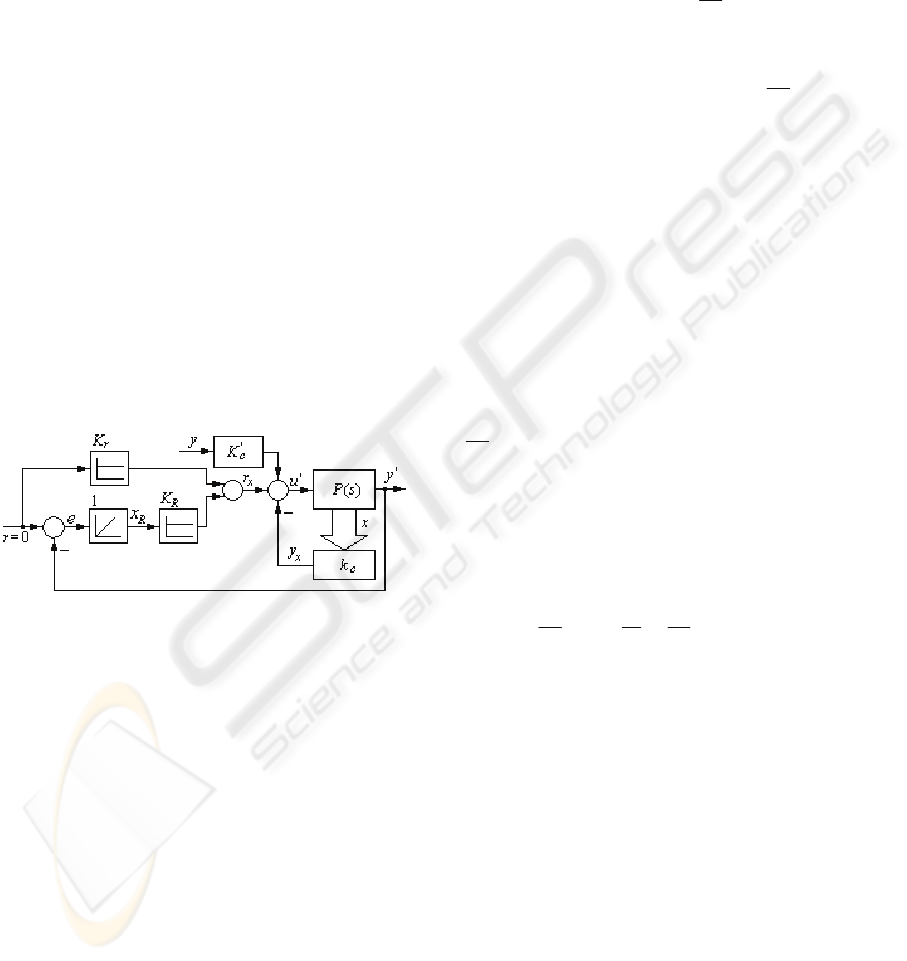
presented in Figure 1. The dotted connection
highlighted is valid only when the experiments
specific to IFT are done. That connection is not
applied during the normal system operation.
Figure 1: IFT-based state feedback control system
structure.
The main variables and blocks illustrated in
Figure 1 represent: IFT – the IFT algorithm, RM –
the reference model,
2
21
][ Rxx
T
∈=x
– the state
vector (T highlights the matrix transposition),
ICINCO 2009 - 6th International Conference on Informatics in Control, Automation and Robotics
42

][
21
KK
c
=k
– the state feedback gain matrix,
)()(
,
sPsP
uα
=
– the transfer function of the
controlled process when the controlled output is
y=x
1
, r – the reference input, e=r–y – the control
error. The other variables will be presented in the
sequel.
If the state feedback gain matrix is regarded as a
controller, then use will be made of its parameters to
minimize the tracking error e
t
between the system
output y and the reference model output y
d
. Let J be
a simple objective function defined over a finite time
horizon N:
∑
=
=
N
t
t
e
N
J
1
2
))((
2
1
)( ρρ
,
(3)
where
m
R∈ρ
is the parameters vector containing at
least the parameters of k
c
and e
t
is the tracking error:
d
t
yye −= )()( ρρ
.
(4)
The IFT results (Hjalmarsson et al., 1994, 1998;
Pfeiffer et al., 2006) are employed to find the
solution ρ
*
to the optimization problem
)(minarg
*
ρρ J
SD∈ρ
=
,
(5)
where several constraints can be imposed regarding
the process and the closed-loop system. One
constraint concerns the stability of the system and
SD represents the stability domain (Precup et al.,
2008).
Solving the optimization problem (5) requires
finding the parameters vectors that make the
gradient equal to zero:
0]...[
1
=
ρ∂
∂
ρ∂
∂
=
∂
∂
T
m
JJJ
ρ
.
(6)
Making use of (3) and (4) the equation (6) will be
transformed into
0])([
1
1
=−
∂
∂
∑
=
N
t
d
T
yy
y
N
ρ
ρ
.
(7)
The partial derivatives
i
y
ρ∂
∂
should be calculated
to obtain the components of the gradient,
i
J
ρ∂
∂
,
mi ,1=
. The new IFT approach to be described as
follows will employ specific experiments to obtain
those components. Use will be made of the
following notation:
i
ρ∂
α
∂
=α'
(8)
to highlight the partial derivative of the variable α
taken with respect to ρ
i
and obtain the simplicity of
the presentation.
The state-space model (1) can be reconsidered by
including one additional state variable to the state
variable. That variable is x
3
=x
R
and it corresponds to
the integrator inserted into the control system
structure. Thus its gain K
R
will be subject to IFT as it
is shown in Figure 1. The extended state-space
model of the process is
⎥
⎥
⎥
⎦
⎤
⎢
⎢
⎢
⎣
⎡
=
⎥
⎥
⎥
⎦
⎤
⎢
⎢
⎢
⎣
⎡
⎥
⎥
⎥
⎥
⎦
⎤
⎢
⎢
⎢
⎢
⎣
⎡
+
+
⎥
⎥
⎥
⎦
⎤
⎢
⎢
⎢
⎣
⎡
⎥
⎥
⎥
⎥
⎦
⎤
⎢
⎢
⎢
⎢
⎣
⎡
−
−−−=
⎥
⎥
⎥
⎦
⎤
⎢
⎢
⎢
⎣
⎡
R
r
s
s
R
Rss
s
s
R
x
I
y
y
y
rK
T
K
x
KKKK
T
KK
x
ω
α
ω
α
ω
α
3
3
2
1
21
1
0
001
1
010
,
(9)
where the parameter K
r
is not included in the tuning
scheme. Its value is set prior to the application of
IFT. One way to choose K
r
is to keep a connection
between the steady-state value of r and the steady-
state value of r
x
for which the desired r can be
tracked by the steady-state value of y. That value of
r
x
can be subject to the experimental identification of
the state feedback control system.
The preparation of the experimental scheme
needed in the calculation of the gradient starts with
the reconsideration of the input-output relations
specific to the control system structure presented in
Figure 1. Observing that generally
xIyykxk
P
y
3
for =−=−=
=
cxcx
rru
u
,
(10)
the following relationships hold:
T
R
T
ERc
Ecr
RRrRRrx
xxKKK
rKxKxK
xKrKuxKrKr
][],[
,
,
21
2211
=−−=
+=−−
−+
=
+
=
xK
xK
.
(11)
Next the gradient of y with respect to each
parameter can be calculated, where the parameters
are the m=3 components of the parameters vector
T
R
KKK ][
21
=ρ
.
(12)
ITERATIVE FEEDBACK TUNING APPROACH TO A CLASS OF STATE FEEDBACK-CONTROLLED SERVO
SYSTEMS
43
Since y and u are functions of ρ it is justified to
apply
'' uPy =
,
(13)
leading to
'''
EcEc
u xKxK +=
.
(14)
In addition, accepting the MIMO formalism
suggested in (10), the following relationship can be
expressed:
''' yKyK
cc
u +=
.
(15)
Equation (15) is of great importance for the new
approach. The first term in the right-hand side of
(15),
yK '
c
, needs to be added to the control signal
to obtain the desired experimental scheme. That
term contains the unmodified output vector (in the
MIMO framework) so the idea is to obtain it from
one first initial experiment (Hjalmarsson et. al.,
1998). The second term in the right-hand side,
'yK
c
, is measured from the control system
structure. Therefore the experimental scheme to
calculate the gradients results in terms of Figure 2
(without the blocks RM and IFT for the sake of
simplicity).
Figure 2: Experimental scheme to calculate the gradients
in the IFT-based state feedback control system structure.
The block
'
c
K
in Figure 2 plays the role of filter.
It differs from one experiment to another one
depending on the actual parameter with respect to
which the gradient is computed.
Since the calculation of the gradients has been
derived in the MIMO framework, m+1=4
experiments are done with it. The first experiment,
referred to also as the normal one, is done with the
control system structure presented in Figure 1 in
order to measure the controlled output y. The next
m=3 experiments, called the gradient experiments,
are done with the experimental scheme presented in
Figure 2. These experiments are done separately for
each parameter in K
c
(defined in (11)) considering
the zero values of the other m–1=2 parameters
(because their derivatives with respect to the current
parameter are zero).
Once the experiments are done the parameters
vector must be updated. Newton’s algorithm is
generally used as one convenient technique which
iteratively approaches a zero of a function without
knowledge of it’s expression. The update law to
calculate the next parameters vector
1+i
ρ
is
)]([
1
1 i
ii
ii
J
est ρ
∂
∂
γ−=
−
+
ρ
Rρρ
,
(16)
where i is the index of the current iteration /
experiment,
i
γ
is the step size,
)]([
i
J
est ρ
∂
∂
ρ
is the
estimate of the gradient, and the regular matrix R
i
can be the estimate of the Hessian matrix (positive
definite) or the identity matrix. The identity matrix is
employed when simple implementations are needed.
Making use of all aspects presented before the
new IFT algorithm consists of the following steps to
be performed per iteration:
Step 1. Do the normal experiment and measure y
based on the control system structure presented in
Figure 1. Next do the three gradient experiments
making use of the experimental scheme presented in
Figure 2 and measure the closed-loop system output
that gives the gradient of the controlled output,
'y
ρ
y
=
∂
∂
.
Step 2. Calculate the output of the reference
model, y
d
, in terms of the control system structure
presented in Figure 3.
Step 3. Calculate the estimate of the gradient of
the objective function:
∑
=
−
∂
∂
=ρ
∂
∂
N
t
d
T
i
N
J
est
1
])([
1
)]([ yρy
ρ
y
ρ
.
(17)
Step 4. Calculate the next set of parameters
1+i
ρ
according to the update law (16).
Three aspects can be highlighted with respect to
the above presented IFT algorithm. First, prior to the
four steps the designer should set the step size, the
reference model and the initial controller parameters
in the vector
0
ρ
. Second, the first task of the state
feedback controller is to ensure an initially stable
control system. The pole placement design can be
used with this regard. Third, the estimate of the
Hessian matrix should be calculated in the step 3 is
it is used as the matrix R
i
in the update law (16) or
an additional experiment can be employed with this
regard.
ICINCO 2009 - 6th International Conference on Informatics in Control, Automation and Robotics
44

3 ACTUATOR SATURATION
PROBLEM
In many cases the actuator is characterized by a
nonlinear input-output map caused by the actuator
saturation. That is a problem because it introduces
usually nonlinear behaviours in the evolution of the
process. Hence it should be avoided. When making
use of the integrator in the controller the actuator
saturation problem becomes important since the
actuator that enters a deep saturation region requires
usually a longer time to re-enter the active region of
normal operation.
Analyzing the structure illustrated in Figure 2
and used in the gradient experiments it is clear that
when the state vector is injected in the control signal
it may cause saturation. Hence the experiment will
be prevented from calculating the correct gradients.
In the following, an actuator with the active input
range varying from −1 to +1 is considered.
One solution to cope with the above mentioned
problem is to design the experiment in such a
manner that the actuator never enters saturation. For
this, the injected quantity must be in the active
region of the actuator’s input-output static map. The
quantity can be scaled to its maximum value from its
evolution. That is obtained by dividing every sample
to the maximum absolute value from the sample
vector. So it is guaranteed that the new quantity to
be injected will be within the accepted domain of the
actuator input.
It can be shown as follows how the gradient
experiments will be influenced. The general case of
MIMO IFT will be considered. First, the scaled,
added value to the control is defined as
|)(|max ,/)()(
,1
tzMMtztz
Nk
s
=
=
=
.
(18)
Next the gradient of the control signal with respect
to the parameters vector,
'u
, can be expressed in
(19) accepting a MIMO control loop with the
controller transfer function C:
'')('' CyzCyyrCu −=−−=
.
(19)
Equation (19) is divided by M resulting in the
following relationship between the scaled values of
the gradients,
Muu
s
/'' =
and
Myy
s
/'' =
:
'/'
ss
CyMzu −=
.
(20)
Concluding, dividing (13) by (18) the result will
be
''
ss
Puy =
.
(21)
Practically a scaled value of the estimate of the
gradient can be obtained making use of the (20) and
(21). After the gradient experiments are done the
measured values
'
s
y
are multiplied by M. Thus they
will give the normal estimate of the gradient to be
used in the iterative minimization of the objective
function J.
4 CASE STUDY AND REAL-TIME
EXPERIMENTS
The validation of the theoretical approaches is done
in terms of a case study consisting of a position
control, y=α, of a DC servo system with backlash.
The experimental setup illustrated in Figure 3 is
built starting with the INTECO DC motor laboratory
equipment. It makes use of an optical encoder for
the angle measurement and a tacho-generator for the
measurement of the angular speed. The tacho-
generator measurements are very noisy. The speed
can also be observed from the angle measurements.
The control system performance indices such as
settling time and overshoot can be assessed easily.
The process (1) is characterized by the
parameters
88.139
=
s
K
and
s 9198.0=
s
T
, obtained
after experimental identification. The initial
parameters vector has been set to
T
]005.00126.00132.0[
0
=ρ
which has been
obtained to stabilize the system.
A constant reference input has been applied,
rad 150
=
r
. This allows, without any loss of
generality, to pre-tune the parameter K
r
at the value
0133.0
=
r
K
and drop it of the variables in the
optimization problem (5). That value of K
r
has been
obtained by steady-state calculation as a gain that
connects r with α through the steady-state gain of
the inner state-feedback loop. The sampling period
has been set to 0.01 s. The following reference
model has been considered:
)15.1/(1)(
2
++= sssG
RM
.
(22)
Figure 3: Experimental setup.
ITERATIVE FEEDBACK TUNING APPROACH TO A CLASS OF STATE FEEDBACK-CONTROLLED SERVO
SYSTEMS
45
Its corresponding pulse transfer function has been
obtained for the accepted sampling period. The
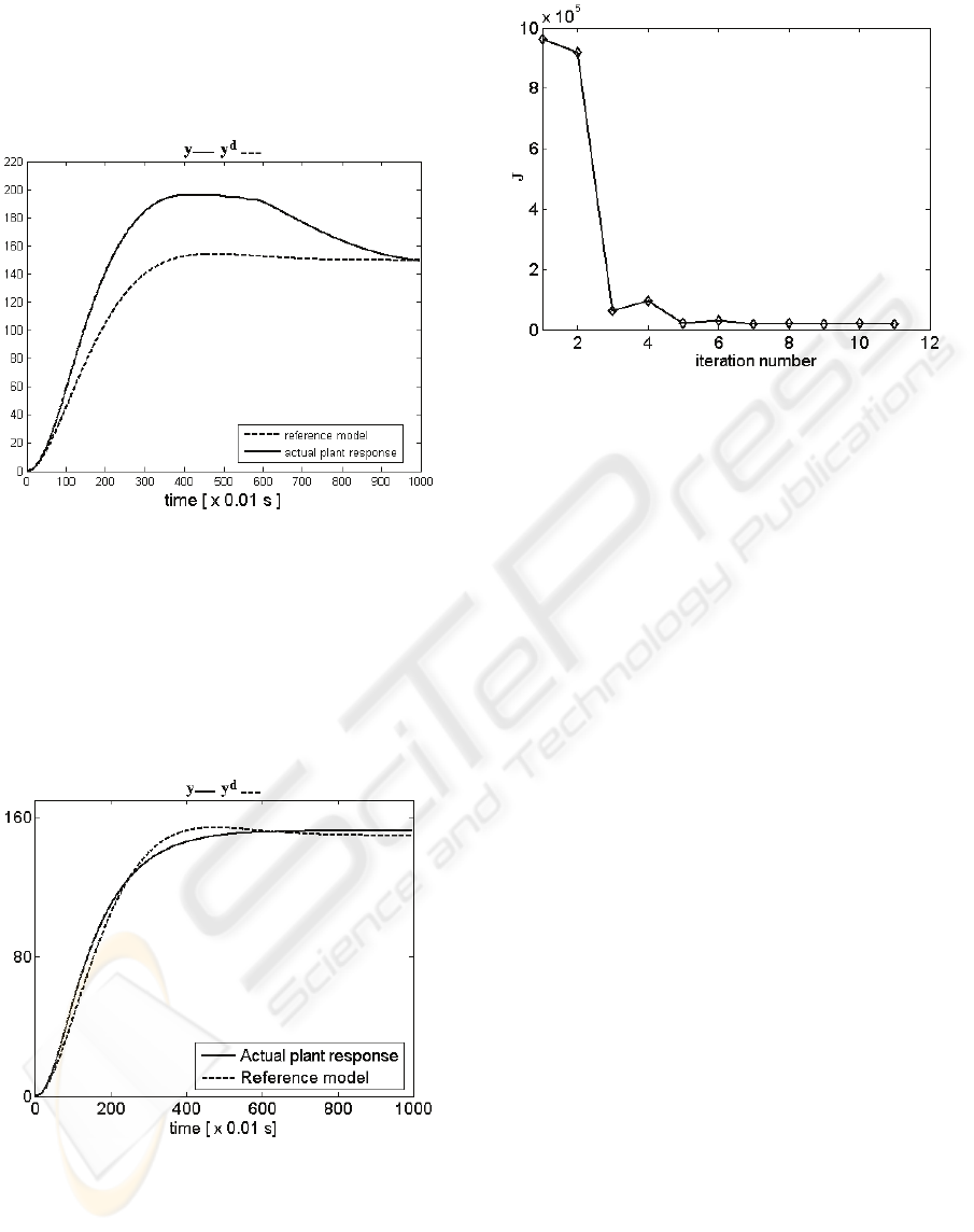
behaviour of the control system before the
application of the IFT algorithm is illustrated in
Figure 4.
Figure 4: Reference model output and controlled output
(position) versus time before IFT.
The IFT algorithm has been applied according to
the steps presented in Section 3. The parameters
have been set to
0001.0=γ
i
and
3
IR
i
=
. The
behaviour of the control system after 12 iterations is
presented in Figure 5. The control system
performance enhancement is highlighted. It is
reflected by smaller overshoot and settling time.
Figure 5: Reference model output and controlled output
(position) versus time after IFT.
The variation of the objective function versus the
iteration number is illustrated in Figure 6. It shows a
good decrease of the objective function and the fact
that the number of iterations can be even smaller.
Figure 6: Objective function versus iteration number.
5 CONCLUSIONS
The paper has been presented a new approach to the
IFT-based design of state feedback control systems
meant for a class of second-order systems with
integral component. The new IFT algorithm can be
applied without any difficulties to the state feedback
control of systems of arbitrary order.
The case study accompanied by real-time
experimental results validates the theoretical
approaches. The control system designed exhibits
better performance indices compared to the situation
prior to the application of the IFT algorithm.
The static and kinetic frictions were neglected.
They can result in the nonlinearity of the input-
output static map
)(uf
=
ω
. The idealization
considered here simplifies the model to be handled
easily because the nonlinearity is not strong.
The first limitation of the proposed IFT approach
concerns the tuning of the initial parameters of the
controller (grouped in the vector
0
ρ
). That problem
is not simple if nonlinear processes are involved.
The second limitation is that the global optimum
cannot be guaranteed. Hence only quasi-optimal
state feedback control systems can be designed.
The presence of the parameter K
r
presented in
Figure 1 and Figure 2 is not mandatory because the
integrator acts in the direction of error alleviation.
So the control system structure can be simplified.
However its presence is important because it can
influence the initial control error with effects on the
convergence of the IFT algorithm.
The future research will be focused on: the
consideration of more complex objective functions
to include the control signal, the state and output
ICINCO 2009 - 6th International Conference on Informatics in Control, Automation and Robotics
46

sensitivity functions as well, the generalization to
nonlinear processes (Cottenceau et al., 2001;
Johanyák and Kovács, 2007; Savaresi et al., 2006;
Andrade-Cetto and Thomas, 2008; Giua and Seatzu,
2008; Precup et al., 2008a; Dolgui et al., 2009)
including MIMO servo systems, and the mapping of
the results from the linear case onto the parameters
of the fuzzy controllers in the framework of state
feedback fuzzy control systems. The convergence
analysis of all IFT algorithms is needed.
ACKNOWLEDGEMENTS
The paper was supported by the CNMP & CNCSIS
of Romania. The first and fifth authors are doctoral
students with the “Politehnica” University of
Timisoara, Romania, and also SOP HRD
stipendiaries co-financed by the European Social
Fund through the project ID 6998.
REFERENCES
Andrade-Cetto, J., Thomas, F., 2008. A wire-based active
tracker. IEEE Transactions on Robotics. 24, 642-651.
Åström, K. J., Hägglund, T., 2000. Benchmark systems for
PID control. In Preprints of IFAC PID’00 Workshop.
Terrassa, Spain, 181-182.
Barut, M., Bogosyan, S., Gokasan, M., 2008.
Experimental evaluation of braided EKF for sensorless
control of induction motors. IEEE Transactions on
Industrial Electronics. 55, 620-632.
Costas-Perez, L., Lago, D., Farina, J., Rodriguez-Andina,
J. J., 2008. Optimization of an industrial sensor and
data acquisition laboratory through time sharing and
remote access. IEEE Transactions on Industrial
Electronics. 55, 2397-2404.
Cottenceau, B., Hardouin, L., Boimond, J.-L., Ferrier, J.-
L., 2001. Model reference control for timed event
graphs in dioids. Automatica. 37, 1451-1458.
Denève, A., Moughamir, S., Afilal, L., Zaytoon, J., 2008.
Control system design of a 3-DOF upper limbs
rehabilitation robot. Computer Methods and Programs
in Biomedicine. 89, 202-214.
De Santis, A., Siciliano, B., Villani, L., 2008. A unified
fuzzy logic approach to trajectory planning and
inverse kinematics for a fire fighting robot operating in
tunnels. Intelligent Service Robotics. 1, 41-49.
Dolgui A., Guschinsky, N., Levin, G., 2009. Graph
approach for optimal design of transfer machine with
rotary table. International Journal of Production
Research. 47, 321-341.
Giua, A., Seatzu, C., 2008. Modeling and supervisory
control of railway networks using Petri nets. IEEE
Transactions on Automation Science and Engineering.
6, 431-445.
Gomes, L., Costa, A., Barros, J. P., Lima, P., 2007. From
Petri net models to VHDL implementation of digital
controllers. In Proceedings of 33
rd
Annual Conference
of the IEEE Industrial Electronics Society (IECON
2007). Taipei, Taiwan, 94-99.
Hjalmarsson, H., 1999. Efficient tuning of linear
multivariable controllers using Iterative Feedback
Tuning. International Journal of Adaptive Control and
Signal Processing. 13, 553-572.
Hjalmarsson, H., Birkeland, T., 1998. Iterative Feedback
Tuning of linear time-invariant MIMO systems. In
Proceedings of 37
th
IEEE Conference on Decision and
Control. Tampa, FL, 3893-3898.
Hjalmarsson, H., Gevers, M., Gunnarsson, S., Lequin, O.,
1998. Iterative Feedback Tuning: theory and
applications. IEEE Control Systems Magazine. 18, 26-
41.
Hjalmarsson, H., Gunnarsson, S., Gevers, M., 1994. A
convergent iterative restricted complexity control
design scheme. In Proceedings of 33
rd
IEEE
Conference on Decision and Control. Lake Buena
Vista, FL, 1735-1740.
Horváth, L., Rudas, I. J., 2004. Modeling and Problem
Solving Methods for Engineers. Burlington, MA:
Academic Press, Elsevier.
Isermann, R., 2003. Mechatronic Systems: Fundamentals.
Berlin, Heidelberg, New York: Springer-Verlag.
Jansson, H., Hjalmarsson, H., 2004. Gradient
approximations in Iterative Feedback Tuning for
multivariable processes. International Journal of
Adaptive Control and Signal Processing. 18, 665-681.
Johanyák, Z. C., Kovács, S., 2007. Sparse fuzzy system
generation by rule base extension. In Proceedings of
11
th
International Conference on Intelligent
Engineering Systems (INES 2007). Budapest,
Hungary, 99-104.
Kovács, G. L., 2006. Management and production control
issues of distributed enterprises. In Proceedings of
PROLAMAT 2006 IFIP TC5 International
Conference. Shanghai, China, 11-20.
Orlowska-Kowalska, T., Szabat, K., 2008. Damping of
torsional vibrations in two-mass system using adaptive
sliding neuro-fuzzy approach. IEEE Transactions on
Industrial Informatics. 4, 47-57.
Petres, Z., Baranyi, P., Korondi, P., Hashimoto, H., 2007.
Trajectory tracking by TP model transformation: case
study of a benchmark problem. IEEE Transactions on
Industrial Electronics. 54, 1654-1663.
Pfeiffer, D., Stephens, R. I., Vinsonneau, B., Burnham, K.
J., 2006. Iterative Feedback Tuning applied to a ship
positioning controller. In Proceedings of 18
th
International Conference on Systems Engineering
(ICSE 2006). Coventry, UK, 353-358.
Precup, R.-E., Preitl, S., Fodor, J., Ursache, I.-B., Clep, P.
A., Kilyeni, S., 2008a. Experimental validation of
Iterative Feedback Tuning solutions for inverted
pendulum crane mode control. In Proceedings of 2008
Conference on Human System Interaction (HSI 2008).
Krakow, Poland, 536-541.
Precup, R.-E., Preitl, S., Rudas, I. J., Tomescu, M. L., Tar,
ITERATIVE FEEDBACK TUNING APPROACH TO A CLASS OF STATE FEEDBACK-CONTROLLED SERVO
SYSTEMS
47

J. K., 2008b. Design and experiments for a class of fuzzy
controlled servo systems. IEEE/ASME Transactions
on Mechatronics. 13, 22-35.
Savaresi S. M., Tanelli, M., Taroni, F., Previdi, F. Bittanti,
S., Prandoni, V., 2006. Analysis and design of an
automatic motion-inverter. IEEE/ASME Transactions
on Mechatronics. 11, 346-357.
Škrjanc, I., Blažič, S., Agamennoni, O., 2005. Interval
fuzzy model identification using l
∞
-norm. IEEE
Transactions on Fuzzy Systems, 13, 561-568.
Vaščák, J., 2008. Fuzzy cognitive maps in path planning.
Acta Technica Jaurinensis, Series Intelligentia
Computatorica. 1, 467-479.
ICINCO 2009 - 6th International Conference on Informatics in Control, Automation and Robotics
48
