COMPUTATIONAL ALGORITHM FOR NONPARAMETRIC
MODELLING OF NONLINEARITIES IN HAMMERSTEIN SYSTEMS
Przemysław
´
Sliwi
´
nski and Zygmunt Hasiewicz
Institute of Computer Engineering, Control and Robotics, Wrocław University of Technology
W. Wyspia
´
nskiego 27, Wrocław, Poland
Keywords:
Hammerstein system, Non-parametric identification, Orthogonal expansions, Regression estimation, Compu-
tational algorithm.
Abstract:
In the paper a fast computational routines for identification algorithms for recovering nonlinearities in Ham-
merstein systems based on orthogonal series expansions of functions are proposed. It is ascertained that both,
convergence conditions and convergence rates of the computational algorithms are the same as their much
less computationaly attractive ’theoretic’ counterparts. The generic computational algorithm is derived and
illustrated by three examples based on standard orthogonal series on interval, viz. Fourier, Legendre, and Haar
systems. The exemplary algorithms are presented in a detailed, ready-to-implement, form and examined by
means of computer simulations.
1 INTRODUCTION
Recursive routines for nonparametric identification
are of interest for practitioners mainly because the
recursive formulas, involving only the last estimate
value and/or the current measurements, are much sim-
pler and much less computationally demanding than
their closed-form counterparts, and hence, they seem
to be more suitable for applications with limited com-
putational capabilities (e.g. in power constrained mo-
bile and/or remote devices).
The advantages of the recursive orthogonal series
identification algorithms presented here may thus be
of importance for a wide range of prospective users,
since Hammerstein systems (i.e. the cascades of non-
linear static element followed by the linear dynamics;
Fig. 1) are a popular modelling tool in many fields,
see (Giannakis and Serpedin, 2001); e.g. in biocy-
bernetics: (Westwick and Kearney, 2001; Dempsey
and Westwick, 2004; Kukreja et al., 2005), chem-
istry: (Eskinat et al., 1991), control: (Lin, 1994; Zi-
Qiang, 1993; Zhu and Seborg, 1994), and in econ-
omy: (Capobianco, 2002).
In the paper the new fast routine for a generic or-
thogonal series algorithm modelling a nonlinear char-
acteristic in Hammerstein systems is proposed and
three examples, employing representative orthogonal
bases on intervals, are presented. Namely, the follow-
ing algorithms are provided in a unified and ready-to-
implement form:
• the Fourier trigonometric,
• the Legendre polynomial, and
• the Haar wavelet algorithm.
Nonparametric estimates
1
are well known for their
flexibility. They allow to model virtually any non-
linearity – be it continuous or not – exploiting the
measurement set only, see e.g. (H
¨
ardle, 1990; Gy
¨
orfi
et al., 2002). Application of orthogonal series, in par-
ticular, enables evaluation of the estimates values in
arbitrary points and at any stage of the identification
process (in contrast to kernel-based recursive algo-
rithms when the estimation points need to be set be-
forehand; see e.g. (Greblicki and Pawlak, 1989)).
2 REFERENCE ALGORITHM
The Hammerstein system under consideration is de-
scribed by the discrete-time input-output equation
y
k
=
∑
i=0,1,...
λ
i
m(x
k−i
) + z
k
(1)
where m(x) is the system nonlinearity,
{
λ
i
}
is the im-
pulse response of the dynamic subsystem, and z
k
is
1
The term ’nonparametric’ refers to the a priori knowl-
edge which is at ones disposal rather to the form of the re-
sulting algorithm.
116
´
Sliwi
´
nski P. and Hasiewicz Z. (2009).
COMPUTATIONAL ALGORITHM FOR NONPARAMETRIC MODELLING OF NONLINEARITIES IN HAMMERSTEIN SYSTEMS.
In Proceedings of the 6th International Conference on Informatics in Control, Automation and Robotics - Signal Processing, Systems Modeling and
Control, pages 116-123
DOI: 10.5220/0002207301160123
Copyright
c
 SciTePress

the external, additive noise. The standard nonpara-
metric assumptions are imposed on the system char-
acteristics, input signals and external noise; cf. (Gre-
blicki and Pawlak, 1994; Greblicki and Pawlak, 2008;
´
Sliwi
´
nski et al., 2009):
1. An input signal,
{
x
k
}
, and an external noise,
{
z
k
}
, are second-order random stationary pro-
cesses. They are mutually independent and the
latter is a zero-mean process. The input
{
x
k
}
is
white and has density, f (x), strictly positive in the
identification interval, say a standard unit interval,
[0,1].
2. A nonlinear characteristic of the static system,
m(x), has ν derivatives.
3. A linear dynamic subsystem is asymptotically sta-
ble. Its impulse response,
{
λ
i
}
, i = 0,1,..., is un-
known.
4. A set,
{
(x
l
,y
l
)
}
, l = 1, 2, . ..,k,... of the system
input and output measurements is available.
m(x)
{}
i
¸
x
k
y
k
z
k
Figure 1: The identified Hammerstein system.
Remark 1. Due to a composite structure of Ham-
merstein systems, only a scaled and shifted version
of the characteristic m (x) of the static block, i.e. the
nonlinearity µ (x) = am(x) + b, where a = λ
0
6= 0,
b = Em(x
1
)
∑
∞
i=1
λ
i
, can at most be recovered from
the input-output measurements. Indeed, the following
holds, cf. (1) and (Greblicki and Pawlak, 2008):
E (y
k
|
x
k
= x ) = λ
0
m(x) + Ez
k
+E
∑
i=1,...
λ
i
m(x
k−i
)
= λ
0
m(x) + b
and to recover the genuine m(x) in general case, one
needs an additional a priori information about the
nonlinearity, e.g. its value in some points.
The reference algorithm construction starts with
the observation that any square integrable function in
the unit interval [0,1] may be represented by the or-
thogonal series (expansion):
µ(x) =
∞
∑
m=0
α
m
φ
m
(x) (2)
where
{
φ
m
}
, m = 0,1,... is a proper orthonormal ba-
sis on the interval [0,1], and where
α
m
=
h
φ
m
,µ
i
=
Z
1
0
φ
m
(x)µ (x)dx (3)
are the expansion (generalized Fourier) coefficients
associated with φ
m
’s. Let µ
m
(x) be an m-term ap-
proximation (cut-off) of µ(x), that is, let (cf. (2))
µ
m
(x) =
m
∑
m=0
α
m
φ
m
(x). (4)
Due to the completeness of the basis
{
φ
m
}
we have
Z
1
0
[µ(x) −µ
m
(x)]
2
dx → 0 as m → ∞
for virtually any µ (x); cf. (2). Moreover, due to
orthogonality of
{
φ
m
}
, the approximation accuracy
grows with the increasing number of approximation
terms, m, as the approximation error is
∑
∞
m=m+1
α
2
m
.
Assume now that for any k, the earlier and present
measurements {(x
l
,y
l
)}, l = 1,...,k, are sorted (or-
dered) increasingly with respect to the input values x
l
.
Then, the orthogonal series reference algorithm may
have the following natural form (cf. (4))
¯µ
m
(x) =
m
∑
m=0
¯
α
m
φ
m
(x) (5)
where (cf. (3) and see (Greblicki and Pawlak, 1994;
Greblicki and Pawlak, 2008))
¯
α
m
=
k
∑
l=1
y
l
Z
x
l
x
l−1
φ
m
(u)du (6)
are estimates of the true expansion coefficients α
m
(with x
0
= 0). The following theorem describes the
limit properties of the reference algorithm:
Theorem 1. If the number m of terms in (5), i.e. the
number of the estimated coefficients
¯
α
m
in the algo-
rithms, increases with the measurements number k so
that
m → ∞ and m/k →0 as k → ∞,
then
E
Z
1
0
[µ(x) − ¯µ
m
(x)]
2
dx → 0 as k → ∞.
Moreover, for Fourier and Legendre series the algo-
rithm attains, for m =
j
k
1/(2ν+1)
k
, the best possible
asymptotic convergence rate, i.e. for any ε > 0, it
holds for them that
E
Z
1−ε
ε
[µ(x) − ¯µ
m
(x)]
2
dx = O

k
−2ν/(2ν+1)

while the convergence of the Haar series algorithm
achieves, for m =

k
1/3

, the asymptotic rate
E
Z
1
0
[µ(x) − ¯µ
m
(x)]
2
dx = O

k
−2/3

for any ν = 1,2,....
COMPUTATIONAL ALGORITHM FOR NONPARAMETRIC MODELLING OF NONLINEARITIES IN
HAMMERSTEIN SYSTEMS
117

Proof. The proofs of the theorem for the algorithms
with Fourier trigonometric and Legendre polynomial
bases can be found in (Greblicki and Pawlak, 1994)
and in (Greblicki and Pawlak, 2008). The proof for
Haar wavelet algorithm is in (Greblicki and
´
Sliwi
´
nski,
2002).
Remark 2. Using sorted measurements results in
a non-quotient form of the identification algorithms.
Such a form (achieved at a moderate cost of keep-
ing the measurement data sorted) can be seen as su-
perior to the alternate quotient-form estimates from
the stability and numerical error standpoint, espe-
cially, when the number of measurement data is
small or moderate (see (
´
Sliwi
´
nski, 2009a;
´
Sliwi
´
nski,
2009b) for on-line and e.g. (Greblicki, 1989; Pawlak
and Hasiewicz, 1998; Hasiewicz, 1999; Hasiewicz,
2001; Hasiewicz et al., 2005) for off-line quotient or-
thogonal series algorithms). The orthogonal series
algorithm (5)-(6) were presented in (Greblicki and
Pawlak, 1994).
3 COMPUTATIONAL (FAST)
ALGORITHM
In a view of Theorem 1, the algorithm (5)-(6) pos-
sesses desirable theoretical properties. It however
seems not to be computationally attractive for the fol-
lowing two reasons:
• calculating coefficient estimates needs integra-
tion, and
• updating the estimates, in case when the new
measurement data appear, requires repeating
the whole computation routine (6) ’right from
scratch’.
Our goal is therefore to make the algorithm com-
putationally efficient without sacrificing its prominent
properties. Namely, the abovementioned numeric
shortcomings maybe circumvented by:
• avoiding explicit integration in favor of subtrac-
tion, and
• providing a computation formula for recursive up-
dating of coefficients estimates.
The goal is accomplished in the following fast
generic routine. The first step is elementary – we
simply apply here The First Fundamental Theorem of
Calculus to get the integration-free counterpart of the
estimate in (6)
¯
α
m
=
k
∑
l=1
y
l
[Φ
m
(x
l
) −Φ
m
(x
l−1
)] (7)
where Φ
m
(x) are the indefinite integrals for the ba-
sis functions φ
m
(x). The second step is described
in the following proposition (being a generalization
of the result presented in (
´
Sliwi
´
nski et al., 2009) for
wavelets).
Proposition 2. Let
¯
α
(k)
m
denote the estimate of the
expansion coefficient α
m
obtained for k measure-
ments. Given the ordered sequence, {(x
1
,y
1
),...,
(x
l
,y
l
),(x
l+1
,y
l+1
),...,(x
k
,y
k
)}, assume that for the
new, (k+1)th measurement pair, (x
k+1
,y
k+1
), it holds
that x
l
< x
k+1
< x
l+1
. Then, (i) the new pair is in-
serted between (x
l
,y
l
) and (x
l+1
,y
l+1
) to maintain the
ascending order of the updated measurement set, and
(ii) the following recurrence formula should be ap-
plied to update the coefficient estimates
¯
α
(k+1)
m
=
¯
α
(k)
m
+ (y
k+1
−y
l+1
) × (8)
×[Φ
m
(x
k+1
) −Φ
m
(x
l
)]
with the initial values
¯
α
(0)
m
= 0, and with the initial
measurements set
{
(0,0),(1,0)
}
.
Proof. The proof is immediate. To derive the recur-
rence formula (8), it suffices to subtract the estimate
in (7), computed for k, from the one obtained for k +1
measurements.
Below we present three examples showing how
to implement Fourier, Legendre, and Haar orthogonal
systems in the general identification routine (5)-(8).
3.1 Fourier Trigonometric Series
Since sequence of trigonometric functions
p
1/2π,
n
p
1/πcos(mu),
p
1/πsin(mu)
o
constitutes, for m = 1, 2, . .., an orthogonal basis on
the interval [−π,π]; cf. (Szego, 1974; Greblicki and
Pawlak, 2008), thus for our identification interval,
[0,1], we need φ
0
(x) = 1 and
φ
2m−1
(x) =
√
2sin((2m −1)πx)
φ
2m
(x) =
√
2cos(2mπx)
for m = 1, 2, . . .. From the above we immediately ob-
tain Φ
0
(x) = x and
Φ
2m−1
(x) = −
κ
2m−1
cos((2m −1)πx)
Φ
2m
(x) =
κ
2m
sin(2mπx)
for m = 1,2,... and κ =
√
2/π.
ICINCO 2009 - 6th International Conference on Informatics in Control, Automation and Robotics
118

3.2 Legendre Polynomial Series
The Legendre polynomials can be defined recursively
as
p
m+1
(x) =
2m+1
m+1
xp
m
(x) +
m
m+1
p
m−1
(x)
for m = 1, 2,... with p
0
(x) = 1, p
1
(x) = x; cf. (Szego,
1974; Greblicki and Pawlak, 2008). They form an
orthonormal basis on the interval [−1,1] with the
weighting function
p
(2m + 1)/2. In our algorithm,
for the unit interval we thus need a slightly reformu-
lated
φ
m
(x) =
√
2m + 1p
m
(2x −1).
The following recurrence formula for primitives of
Legendre polynomials holds (see the derivation in
Proposition 3 in Appendix A).
P
m+1
(x)=κ
m

x
2
−1

p
m
(x)+K
m
P
m−1
(x)
for m = 1,2,..., where κ
m
=
(2m + 1)/((m + 1)(m + 2)), K
m
=
m(m −1)/((m + 1)(m + 2)) and P
0
(x) = x + 1,
P
1
(x) =

x
2
−1

/2. Eventually, we have
Φ
m
(x) =
√
2m+1
2
P
m
(2x −1).
3.3 Haar Wavelet Series
To construct Haar wavelet basis one needs two func-
tions, the father and mother Haar wavelets:
ϕ(x) = I
0≤x<1
(x) and ψ(x) = ϕ(2x) −ϕ(2x −1)
and translations and dilations of the latter, i.e.
ψ
kl
= 2
k/2
ψ

2
k
x −l

where the indices k,l run through the ranges 1,...,
and 0, . . . , 2
k
−1, respectively; cf. e.g. (Wojtaszczyk,
1997). In our case the identification interval, [0,1],
is the native one for Haar system and we can directly
take
φ
0
(x) = ϕ(x) and φ
m
(x) = ψ
kl
(x)
for m = 1,2,..., where
k =
b
log
2
m
c
and l = m mod 2
k
(9)
and where x mod y = x − y ·
b
x/y
c
denotes standard
modulus function.
Since, in fact, the father wavelet, ϕ(x), is merely
a box function, then the primitives of basis functions,
φ
m
(x), are simply
Φ
0
(x) = xI
0≤x<1
(x) + I
x≥1
(x)
and
Φ
m
(x) =
1
√
2
k+1
h
Φ
0

2
k+1
x −l

− Φ
0

2
k+1
x −(l + 1)
i
for m = 1, 2, . . . with k, l dependent on m and defined
as in (9).
4 COMPUTATIONAL
COMPLEXITY ANAYSIS
In what follows we compare the computational com-
plexities of both the reference and the proposed fast
computational versions.
4.1 Reference Algorithm
In the reference algorithm implementation one can
naturally distinguish two phases with the main rou-
tine (5)-(6) preceded by sorting of the measurement
sequence. The latter, employing a fast sorting algo-
rithm (e.g. quick sort, heap sort; cf. (Knuth, 1998)),
needs O (k log k) operations.
A naive implementation of the main routine (5)-
(6) requires O (mη) operations in (5) and O (kι) oper-
ations in (6), where O (η) is the cost of evaluating of
φ
m
(x) and where O (ι) is the cost of calculating of the
definite integral for φ
m
(x). The overall cost is there-
fore O (mη ·kι). In a view of Theorem 1 this reads
O

k
1+1/(2q+1)
·ηι

. In case of the Fourier and Haar
algorithms we have O (η) = O (1). In the Legendre al-
gorithm computing φ
m
(x) (i.e. a polynomial of order
m) takes m operations. The cost O (ι) of computing
integrals (since the indefinite integrals for φ
m
(x) are
known) is the same.
Table 1: Complexities of a direct implementation of the ref-
erence algorithms.
Algorithm Cost
Fourier O

k
2
2q+1
(q+1)

Legendre O

k
2
2q+1
(q+2)

Haar O

k
4
3

4.2 Fast Algorithm
Using the above naive implementation results in cost
of at least O

k
2(q+1)/2q+1

operations for every sin-
gle new measurement to be added. Our algorithm
(5), (8) substantially reduces this complexity. First,
searching for the pairs (x
l
,y
l
) and (x
l+1
,y
l+1
) in the
measurement sequence (employing e.g. a standard bi-
nary search algorithm) requires O (log k) operations;
cf. (Knuth, 1998). Computing the updated value
of ¯µ
m
(x) requires another O (m (k)) operations. The
overall cost of the Fourier and Legendre algorithms
(in the latter the recurrence formulas (10), (11) are
COMPUTATIONAL ALGORITHM FOR NONPARAMETRIC MODELLING OF NONLINEARITIES IN
HAMMERSTEIN SYSTEMS
119

used) is therefore of order O (logk) +O (m (k)) =
O(
2q+1
√
k).
In case of the Haar algorithm, this cost can fur-
ther be reduced to the order O (log k) after observa-
tion that, due to compactness of Haar functions sup-
ports, only O(logk) terms of are involved in computa-
tions of (5), (8). Indeed, using wavelet ’natural’ scale-
translation notation (cf. (9)), one can easily ascertain
that, for each scaling index n = 0,...,
b
log
2
m (k)
c
, at
most one function ψ
nl
(x) is non-zero – the one with
translation index l = b2
n
xc. The computation phase
of the Haar algorithm requires thus only O (log k) op-
erations for m = b
3
√
kc.
Table 2: Complexities of fast implementation of the refer-
ence algorithms.
Algorithm Cost
Fourier O

k
1
2q+1

Legendre O

k
1
2q+1

Haar O (log k)
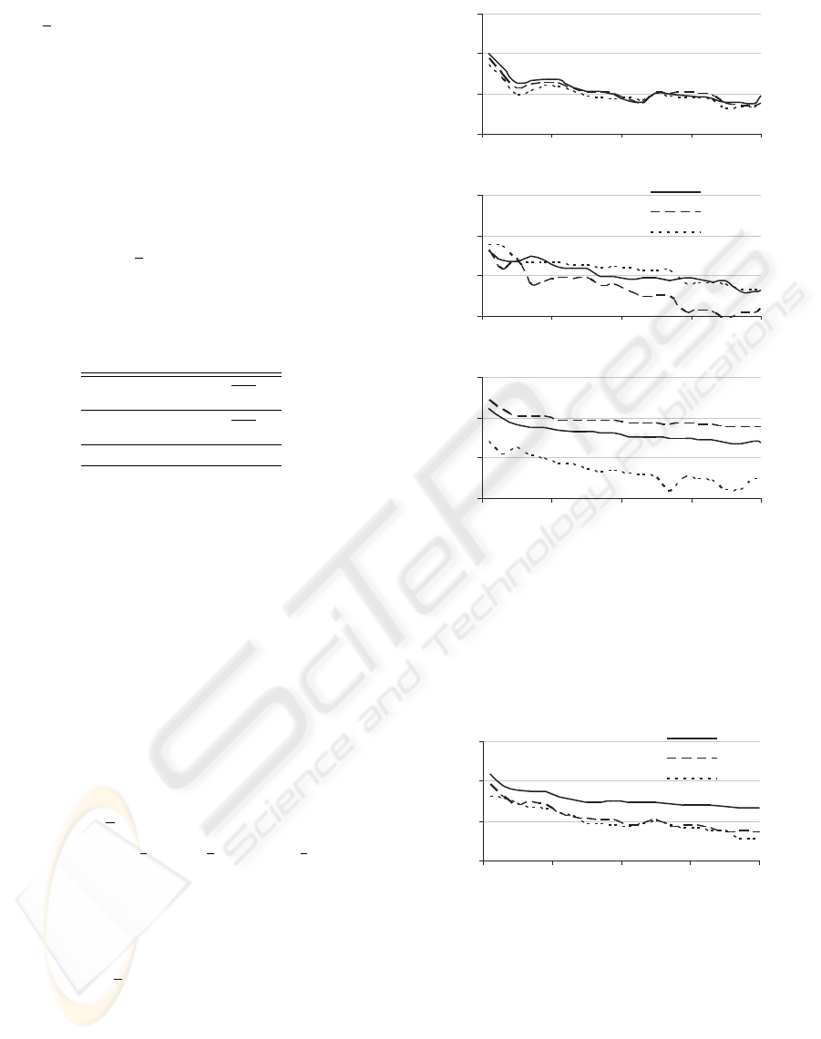
5 NUMERICAL EXPERIMENTS
The first two examples, the Fourier and Legendre al-
gorithms, possess the same asymptotic behavior while
the last, the Haar one, is slightly slower for smooth
nonlinearities (i.e. for ν = 2, 3, . ..). However, as we
will see in the following numerical experiments, this
fact does not necessarily hold true for sample sizes
being small or moderate.
To this end, the following piecewise-
[smooth|linear|constant] characteristics, referred
further to as the root, ramp, and step functions,
respectively, were considered in the interval [0,1]:
m(x) =



3
√
u
2

u +
1
2

I

u +
1
2

+ 2I

u −
1
2

−1
I (u + 1) −I (u)
where u = 2x −1 and I (x) is the abbreviated nota-
tion of the box function I
0≤x<1
(x). The number m of
estimate components, i.e. of coefficients in the algo-
rithms, was governed by the practical rule, according
to which m = b
3
√
kc; cf. (Greblicki and Pawlak, 2008;
Hasiewicz et al., 2005). The input
{
x
l
}
was uniformly
distributed over [0,1], and the (infinite) impulse re-
sponse of the dynamic part was λ
i
= 2
−i
, i = 0,1,...
(thus we had exactly µ(x) = m (x) for all three non-
linearities, cf. Remark 1); the external zero-mean uni-
form noise was set to make max
|
z
l
|
/max
|
m(x)
|
=
10%. Numerically computed MISE error served as
0.001
0.01
0.1
1
0 500 1000 1500 2000
0.001
0.01
0.1
1
0 500 1000 1500 2000
Fourier
Legendre
Haar
0.001
0.01
0.1
1
0 500 1000 1500 2000
k
k
k
Figure 2: The algorithms errors for three test nonlinearities:
a) root, b) ramp, and c) step one.
the indicator of algorithms accuracy (computed in
slightly narrowed interval, [ε,1 −ε] , ε = 0.1, in order
to avoid the boundary effect affecting Fourier algo-
rithm (cf. Figs 2a and 3)).
0.001
0.01
0.1
1
0 500 1000 1500 2000
Fourier
Legendre
Haar
0.001
0.01
0.1
0 500 1000 1500 2000
[GP94]
[SH09]
k
k
Figure 3: Boundary effect illustration.
The experiments unveil that algorithms offer sim-
ilar accuracy for the root function. Slightly better
performance of Legendre algorithm in case of ramp
function and the Haar algorithm in case of step func-
tion can both be attributed to similarity of their basis
functions to the respective nonlinearities. Neverthe-
less, the Haar wavelet algorithm – achieving the simi-
lar results and being much faster – can be pointed out
as the most effective across the whole experiment.
ICINCO 2009 - 6th International Conference on Informatics in Control, Automation and Robotics
120

6 FINAL REMARKS
The new class of fast routines for nonparametric iden-
tification algorithms recovering the nonlinearity in
Hammerstein systems has been proposed. Preserving
all the asymptotic properties of their off-line origins,
the new algorithms offer much more computationally
efficient formulas. Comparing the algorithm proper-
ties one can draw the following conclusions:
• Fourier algorithm is fast but prone to boundary
effect,
• Legendre algorithms is the slowest but free bound-
ary problems, finally
• Haar algorithm is fast but do not perform well in
case of smooth nonlinearities (like the Fourier and
Legendre do).
Remark 3. Owing to the beneficial features pointed
out above it is not a serious disadvantage that all
measurement data need to be kept in our algorithm.
This – admittedly idiosyncratic feature – is a conse-
quence of both the form of the initial off-line version
of the algorithm (6) and the random nature of the in-
put data; cf. (
´
Sliwi
´
nski et al., 2009). Moreover, the
measurement set needs to be maintained only during
the synthesis of the estimate. In the implementation
step, all k measurements can be rid off and only m
coefficients (with m being a significantly smaller num-
ber than k) have to be stored. Observe also that in all
nonparametric algorithms, be them kernel or k −NN
algorithms, see e.g. (Gy
¨
orfi et al., 2002; Greblicki
and Pawlak, 2008), the measurements need to be kept
as well in order to allow computing the estimate value
in arbitrary point.
That the measurements need to be kept in non-
parametric modelling is rather typical as the measure-
ments are essentially the only source of the infor-
mation about the system/phenomenon. This problem
is addressed in (
´
Sliwi
´
nski, 2009a;
´
Sliwi
´
nski, 2009b)
where the quotient form wavelet algorithm is pro-
posed. It is shown there that – on the one hand side –
getting rid of the measurements allows the algorithms
to be asymptotically equivalent to those possessing all
the data, but – on the other – reveals that for small and
moderate measurements number such algorithm per-
form worse.
Finally, we would like to emphasize that the
simplicity of the proposed computational algorithm
should be seen as an advantage for the practitioners
as it allows a straightforward implementation (cf. the
Appendix).
REFERENCES
Capobianco, E. (2002). Hammerstein system representation
of financial volatility processes. The European Physi-
cal Journal B - Condensed Matter, 27:201–211.
Dempsey, E. and Westwick, D. (2004). Identification of
Hammerstein models with cubic spline nonlineari-
ties. IEEE Transactions on Biomedical Engineering,
51(2):237–245.
Eskinat, E., Johnson, S. H., and Luyben, W. L. (1991). Use
of Hammerstein models in identification of non-linear
systems. American Institute of Chemical Engineers
Journal, 37:255–268.
Giannakis, G. B. and Serpedin, E. (2001). A bibliography
on nonlinear system identification. Signal Processing,
81:533–580.
Greblicki, W. (1989). Nonparametric orthogonal series
identification of Hammerstein systems. International
Journal of Systems Science, 20:2355–2367.
Greblicki, W. and Pawlak, M. (1989). Recursive nonpara-
metric identification of Hammerstein systems. Jour-
nal of the Franklin Institute, 326(4):461–481.
Greblicki, W. and Pawlak, M. (1994). Dynamic system
identification with order statistics. IEEE Transactions
on Information Theory, 40:1474–1489.
Greblicki, W. and Pawlak, M. (2008). Nonparametric sys-
tem identification. Cambridge University Press, New
York.
Greblicki, W. and
´
Sliwi
´
nski, P. (2002). Non-linearity esti-
mation in Hammerstein system based on ordered ob-
servations and wavelets. In Proceedings 8th IEEE
International Conference on Methods and Models in
Automation and Robotics – MMAR 2002, pages 451–
456, Szczecin. Institute of Control Engineering, Tech-
nical University of Szczecin.
Gy
¨
orfi, L., Kohler, M., A. Krzy
˙
zak, and Walk, H. (2002).
A Distribution-Free Theory of Nonparametric Regres-
sion. Springer-Verlag, New York.
H
¨
ardle, W. (1990). Applied Nonparametric Regression.
Cambridge University Press, Cambridge.
Hasiewicz, Z. (1999). Hammerstein system identification
by the Haar multiresolution approximation. Interna-
tional Journal of Adaptive Control and Signal Pro-
cessing, 13(8):697–717.
Hasiewicz, Z. (2001). Non-parametric estimation of non-
linearity in a cascade time series system by multiscale
approximation. Signal Processing, 81(4):791–807.
Hasiewicz, Z., Pawlak, M., and
´
Sliwi
´
nski, P. (2005). Non-
parametric identification of non-linearities in block-
oriented complex systems by orthogonal wavelets
with compact support. IEEE Transactions on Circuits
and Systems I: Regular Papers, 52(1):427–442.
Knuth, D. E. (1998). The Art of Computer Programming.
Volume 3. Sorting and searching. Addison-Wesley
Longman Publishing Co., Inc, Boston, MA.
Kukreja, S., Kearney, R., and Galiana, H. (2005).
A least-squares parameter estimation algorithm for
switched Hammerstein systems with applications to
the VOR. IEEE Transactions on Biomedical Engi-
neering, 52(3):431–444.
COMPUTATIONAL ALGORITHM FOR NONPARAMETRIC MODELLING OF NONLINEARITIES IN
HAMMERSTEIN SYSTEMS
121

Lin, S.-K. (1994). Identification of a class of nonlin-
ear deterministic systems with application to manip-
ulators. IEEE Transactions on Automatic Control,
39(9):1886–1893.
Pawlak, M. and Hasiewicz, Z. (1998). Nonlinear system
identification by the Haar multiresolution analysis.
IEEE Transactions on Circuits and Systems I: Fun-
damental Theory and Applications, 45(9):945–961.
´
Sliwi
´
nski, P. (2009a). On-line wavelet estimation of non-
linearities in Hammerstein systems. Part I - algorithm
and limit properties. IEEE Transactions on Automatic
Control. Submitted for review.
´
Sliwi
´
nski, P. (2009b). On-line wavelet estimation of nonlin-
earities in Hammerstein systems. Part II - small sam-
ple size properties. IEEE Transactions on Automatic
Control. Submitted for review.
´
Sliwi
´
nski, P., Rozenblit, J., Marcellin, M. W., and
Klempous, R. (2009). Wavelet amendment of polyno-
mial models in nonlinear system identification. IEEE
Transactions on Automatic Control, 54(4):820–825.
Szego, G. (1974). Orthogonal Polynomials. American
Mathematical Society, Providence, R.I., 3rd edition.
Westwick, D. T. and Kearney, R. E. (2001). Separable least
squares identification of nonlinear Hammerstein mod-
els: Application to stretch reflex dynamics. Annals of
Biomedical Engineering, 29(8):707–718.
Wojtaszczyk, P. (1997). A Mathematical Introduction to
Wavelets. Cambridge University Press, Cambridge.
Zhu, X. and Seborg, D. E. (1994). Nonlinear predictive
control based on Hammerstein system. Control The-
ory Applications, 11:564–575.
Zi-Qiang, L. (1993). Controller design oriented model iden-
tification method for Hammerstein system. Automat-
ica, 29:767–771.
APPENDIX
Recursion in Legendre Polynomials
The well known recurrence relation between Legen-
dre polynomials of adjacent orders (see e.g. (Szego,
1974)), i.e.:
(m + 1) p
m+1
(x) = (2m + 1)xp
m
(x) + mp
m−1
(x)
allows convenient generation of increasing order ele-
ments of polynomial orthogonal basis
p
m+1
(x) =
2m+1
m+1
xp
m
(x) +
m
m+1
p
m−1
(x) (10)
for m = 1,2,..., given p
0
(x) = 1 and p
1
(x) = x.
In the following proposition we show that the sim-
ilar relation holds for primitive functions of these
polynomials.
Proposition 3. Let P
m
(x) =
R
x
−1
p
m
(u)du. The fol-
lowing recurrence relation holds
P
m+1
(x) =
(2m+1)
(
x
2
−1
)
(m+1)(m+2)
p
m
(x) (11)
+
m(m−1)
(m+1)(m+2)
P
m−1
(x)
for m = 1,2,... and with
P
0
(x) = x + 1 and P
1
(x) =
1
2

x
2
−1

.
Proof. We will give only a sketch of the proof as it
involves elementary (yet a bit tedious) calculations.
Integrating both sides of the formula in (10) yields
P
m+1
(x) =
2m+1
m+1
Z
x
−1
up
m
(u)du −
m
m+1
P
m−1
(x) (12)
Employing now integration by parts and another
known recursive formula:

1 −x
2

p
0
m
(x) = m[p
m−1
(x) −xp
m
(x)]
we get
Z
x
−1
up
m
(u)du =
x
2
−1
m+2
p
m
(x) +
m
m+2
P
m−1
(x)
which applied to (12) yields (11), and (after substi-
tution m := m - 1) the formula used in subsequent
C++ implementation.
Code Samples
The following C++ implementations of the presented
recursive formulas prove not to be much more intri-
cate than their mathematical origins in (10):
template <typename T> struct p
{
T operator()(T const &x, size_t m)const
{
T const _2_ = T(2), _1_ = T(1);
if(m == 0) return _1_;
if(m == 1) return x ;
p<T> const lp;
return ((_2_*m-_1_)*x*lp(x, m-1)
- (m-_1_)*lp(x, m-2))/m;
}
};
and in (11), respectively:
template <typename T> struct P
{
T operator()(T const &x, size_t m)const
{
T const _2_ = T(2), _1_ = T(1);
if(m == 0) return x + _1_;
if(m == 1) return (x*x - _1_)/_2_;
ICINCO 2009 - 6th International Conference on Informatics in Control, Automation and Robotics
122

p<T> const lp;
P<T> const lpi;
return ( (_2_*m-_1_)*(x*x-_1_)
* lp(x, m - 1)
+ (m - _1_) * ( m - _2_)
* lpi(x, m - 2))
/(m * (m + _1_));
}
};
COMPUTATIONAL ALGORITHM FOR NONPARAMETRIC MODELLING OF NONLINEARITIES IN
HAMMERSTEIN SYSTEMS
123