SEGMENTS OF COLOR LINES
A Comparison through a Tracking Procedure
Mich
`
ele Gouiff
`
es, Samia Bouchafa
Institut d’Electronique Fondamentale, UMR 8622, Universit
´
e Paris Sud 11, France
Bertrand Zavidovique
Institut d’Electronique Fondamentale, UMR 8622, Universit
´
e Paris Sud 11, France
Keywords:
Computer vision, Color image processing, Level lines, Color lines, Segments features, Tracking, matching.
Abstract:
This paper addresses the problem of visual target tracking by use of robust primitives. More precisely, we
evaluate the use of color segments features in a matching procedure and compare the dichromatic color lines
(Gouiff
`
es and Zavidovique, 2008) with the existing ones, defined in the HSV color space. The motion param-
eters of the target to track are computed through a voting strategy, where each pair of color segments votes first
for one new location, then for two scale changes. Their vote is weighted according to the pairing relevancy
and to their location in the bounding box of the tracked object. The comparison is made in terms of robustness
to color illumination changes and in terms of quality (robustness of the location of the target during the time).
Experiments are carried out on pedestrian and car image sequences. Finally, the dichromatic lines provide
a better robustness to appearance changes with fewer primitives. It finally results in a better quality of the
tracking.
1 INTRODUCTION
Since the last decades, computer vision and im-
age processing assume a particular importance in
robotics. For instance, in the emerging field of intel-
ligent vehicle, the car manufacturers compete to pro-
pose assistance multisensor systems based on lasers
or vision, in order to ensure a better road safety. In
addition to being less and less expensive, vision sen-
sors offer several advantages, the primary of which
is to provide a large amount of information on wide
regions: depth or motion for example.
Motion or stereovision analysis requires a robust
matching of several primitives between two images.
In that context, extracting robust features remains a
key problem.
Indeed, non-stationary visual appearance usually
jeopardizes the matching. Partial occlusions, clutter
of the background or a complicated relative motion
of the object with respect to the camera (in a mov-
ing vehicle for example) are among classical difficul-
ties. Partial occlusions can be dealt with by matching
a large amount of sparse features extracted from ob-
jects, such as points for example (Baker, 2004). In-
deed, it is implausible that the whole features be oc-
cluded simultaneously.
Global features based on color invariants (Gevers
and Smeulders, 1999), or local features like corners,
points, segments, level lines (Caselles et al., 1999) can
answer to the problem of photometric changes. Level
lines are indeed an interesting alternative to edge-
based techniques, since they are closed and less sen-
sitive to external parameters. They provide a compact
geometrical representation of images and they are, to
some extent, robust to contrast changes. For instance,
junctions and segments of level lines have been used
successfully in matching processes in the context of
stereovision for obstacle detection (Suvonvorn et al.,
2007)(Bouchafa and Zavidovique, 2006).
Of course, the choice of the matching strategy has
to be led by the nature of the features. That explains
partly the large amount of tracking methods, among
which correlative and differential methods (Hager and
Belhumeur, 1998)(Jurie and Dhome, 2002), kernel-
based techniques (Comaniciu and Meer, 2002) and
active contours (Paragios and Deriche, 2005) for in-
stance.
This paper compares the robustness of our color
433
Gouiffès M., Bouchafa S. and Zavidovique B. (2009).
SEGMENTS OF COLOR LINES - A Comparison through a Tracking Procedure.
In Proceedings of the 6th International Conference on Informatics in Control, Automation and Robotics - Robotics and Automation, pages 433-438
DOI: 10.5220/0002208504330438
Copyright
c
 SciTePress

segments based on the dichromatic model (Gouiff
`
es
and Zavidovique, 2008) with the luminance and HSV
color lines defined by (Caselles et al., 2002) and (Coll
and Froment, 2000), through an appropriate matching
procedure. This method is designed to robustly track
rigid and non rigid objects in images sequences. The
strategy chosen is based on a weighted voting process
in the space of the motion parameters.
The remainder of the paper is structured as fol-
lows. Section 2 describes the extraction of the color
segments. Then, the matching procedure is explained
in Section 3. To finish, the results of section 4
show the efficiency of the proposed color features for
matching.
2 SEGMENTS OF COLOR LINES
The concept of level lines is recalled in section 2.1.
Then, section 2.2 focuses on the extraction of the seg-
ments. Their characterization is finally described in
section 2.3.
2.1 Color Lines
Let I(p) be the image intensity at pixel p(x,y) of co-
ordinates (x,y). It can be decomposed into upper N
u
or lower N
l
level sets:
N
u
(E) =
{
p,I(p) ≥ E
}
, N
l
(E) =
{
p,I(p) ≤ E
}
(1)
where E denotes the considered level. The topo-
graphic map results from the computation of the level
sets for each E in the gray level range. The level
lines, noted L, are defined as the edges of N and
form a set of Jordan curves. This concept has been
expanded to color in (Coll and Froment, 2000) and
(Caselles et al., 1999). The authors use the HSV color
space, the components of which are less correlated
than RGB’s. Also, this representation is claimed to be
in adequacy with perception rules of the human visual
system. However, they favor the intensity for the def-
inition of the topographic map. Unfortunately, since
the hue is ill-defined with unsaturated colors, this kind
of a representation may output irrelevant level sets,
due to the noise produced by the color conversion at a
low saturation.
More recently, the dichromatic lines have been in-
troduced in (Gouiff
`
es and Zavidovique, 2008). They
are based on the Shafer model which states that the
colors of most Lambertian objects are distributed
along several straight lines in the RGB space, join-
ing the origin (0, 0,0) to the diffuse color components
c
c
c
b
(p). Therefore, while gray level sets are extracted
along the luminance axis of the RGB space, these
color sets are designed along each body (or diffuse)
reflection vector c
c
c
b
. On each of those vectors, a color
can be located by its distance ρ to the origin (the black
color), and each vector is located by its zenithal and
azimuthal angles (θ,φ), in a spherical frame noted
TPR in this paper.
These lines provide a good trade-off between
compactness and robustness to color illuminant
changes. The present evaluation compares the seg-
ments extracted in RGB, HSV and TPR through the
actual and generic application of tracking.
2.2 Extraction of Color Segments
The segment extraction here is an extension to color
of the recursive procedure described in (Bouchafa and
Zavidovique, 2006). It exploits the inclusion property
of the level sets to extract the segments of level lines.
The procedure tracks lines until they split. Along the
search, straight subparts, i.e. segments, are isolated.
The procedure starts at each point p and first deter-
mines which color channel is the most appropriate to
track the line. In this paper, the component k of lowest
contrast is chosen. Indeed, when a color line exists on
this channel, it is likely to exist in both other compo-
nents, and consequently to lay on a real physical con-
tour of the object. This strategy aims at reducing the
extracted noise and the number of segments to match.
Once the channel is chosen in p, we determine iter-
atively which one among p’s 8-connected neighbors
is its successor. Each successor becomes the current
pixel and the procedure repeats until stopping criteria
get true. q is the successor of p when the following
conditions are respected:
1. At least, one line L passes between q and p:
|I(p) − I(q)| ≤ λ.
2. The tracked L of the chosen path belongs to the same
groups of level lines being tracked from the beginning.
3. The interior (vs. exterior) of the corresponding N is
kept on the same side.
4. The tracked level lines remain straight.
For further readings, one can refer to (Bouchafa
and Zavidovique, 2006). At that stage, a set of seg-
ments S =
{
s
i
}
has been extracted from the image.
2.3 Characterization of Color Segments
Fig.1 illustrates the characterization of the segments.
A segment s
i
is characterized geometrically and col-
orimetrically: the coordinates of its central point p
i
=
(x
i
,y
i
), its length l
i
, its angle α
i
, its color. We note
µ
i
L
(k) and µ
i
R
(k), for k = 1..3, the mean color on
channel k, respectively on the left (L) and on the right
hand (R) of the segment s
i
.
ICINCO 2009 - 6th International Conference on Informatics in Control, Automation and Robotics
434

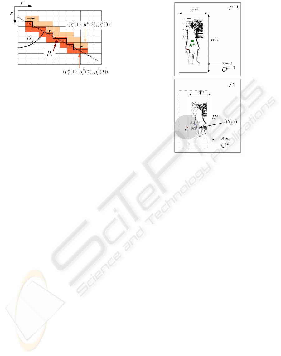
Figure 1: Characterization of the color segment.
The following section describes the matching of
these color features, based on the definition of a sim-
ilarity between color segments.
3 MATCHING AND TRACKING
Be I
t
and I
t−1
two subsequent frames at current and
previous times t and t − 1. Object O at time t, de-
noted as O
t
, is described spatially by its bounding
box BB
t
of height H
t
and width W
t
and its centroid
P
t
, as shown on Fig.2. It can reasonably be selected
through a fast motion analysis scheme (Lacassagne
et al., 2008) for example.
Knowing the previous object O
t−1
in I
t−1
, the
tracking consists in computing its new position in I
t
by matching the segments exhibited according to sec-
tion 2.
As in most non-rigid trackers (Comaniciu and
Meer, 2002), the object motion is assumed a compo-
sition of a translation and two scale changes A
x
and
A
y
along x and y respectively. Since matching is per-
formed between two subsequent frames and suppos-
ing a small relative motion object/camera, we further
assume a low warping of the object. Therefore, we
consider that the new object is located in a search
area V (O
t−1
) which is BB
t−1
enlarged by a factor
x2. We also consider that the scale changes range in
[1 − A,1 + A], where A is the maximum possible per-
centage of scale change.
To secure unambiguous tracking, one needs to
consider a large enough number of pairs together.
In Fig.2, the object is represented by a set of seg-
ments, which are plotted in black. A set of segments
S
t−1
=
{
s
i
}
is extracted in O
t−1
and a set S
t
=

s
j

is extracted in V (O
t−1
). In a first stage, each feature
s
i
is entitled to match with each feature s
j
located in
V (s
i
) in I
t
. The similarity function explained below
evaluates how well features match.
Figure 2: Illustration of the tracking procedure.
3.1 Similarity Function
For all s
i
∈ I
t−1
and all s
j
∈ V (s
i
) ⊂ I
t
(see Fig.2), we
define a similarity function based on a color distance
C
µ
(i, j) and the angle difference C
α
(i, j) ∈ [0,1]:
C
µ
(i, j) = C
0
3
∑
k=1
|µ
L
i
(k) − µ
L
j
(k)| + |µ
R
i
(k) − µ
R
j
(k)|(2)
C
α
(i, j) = (|α
i
− α
j
|
moduloπ
)/π (3)
C
0
is a normalization value which depends on the
dynamics of the image, typically C
0
= 2
N
/6 for an
image coded on N bits. We deduce the following sim-
ilarity function (∈ [0, 1]):
C (i, j) = 1 −a
µ
C
µ
(i, j) − a
α
C
α
(i, j) with a
µ
+ a
α
= 1 (4)
a
µ
and a
α
balance the similarity criteria. The higher
C (i, j), the more similar s
i
and s
j
. In order to reduce
the number of potential matches, two additional crite-
ria have to be met beforehand:
• s
i
and s
j
have comparable sizes so they respect the crite-
rion D
l
: D
l
=

1 when 1 − A ≤ l
j
/l
i
≤ 1 + A, else 0

• s
i
and s
j
have comparable directions so
they respect the criterion D
α
: D
α
=

1 when |α
i
− α
j
|mod
π
< T
α
, else 0

, where T
α
is a threshold, high enough not to be critical.
SEGMENTS OF COLOR LINES - A Comparison through a Tracking Procedure
435

3.2 Computation of the New Object
Location and Scale
The estimation of both centroid and scales relies on a
voting process. Each potential pair of features (s
i
,s
j
),
with s
j
∈ V (s
i
) votes first to one candidate centroid
P
j
, each vote being weighted considering the rele-
vancy of the pairing features. The notion of rele-
vancy translates in terms of the similarity defined in
(2) and in terms of the location of the feature within
BB
t−1
. Indeed, similarly to mean-shift methods (Co-
maniciu and Meer, 2002), a Gaussian weighting func-
tion K(p
i
) is considered for each primitive. In order
to cope with partial occlusions and cluttered back-
ground, a higher confidence is granted to locations p
i
close to the centroid P
t
compared to peripheral ones.
3.2.1 Estimation of the New Location P
t
Each feature s
i
previously extracted on O
t−1
is as-
signed a vector v
i
which goes from p
i
to the previous
centroid P
t−1
such that v
i
= P
t−1
− p
i
. Since small
object motions are conjectured, the scale is assumed
to be constant in a first approximation. Therefore,
if s
i
is correctly matched with s
j
of centroid p
j
, the
candidate centroid P
j
is likely to be located around
p
j
− v
i
. The uncertainty is lifted only in the rare
cases where the object is planar, its motion is strictly
fronto-parallel and its scale does not change. In or-
der to model this uncertainty, a 2D Gaussian function
ε(p,σ
A
) assigns weights at once to P
j
and to few of its
neighbor points. Its standard deviation σ
A
expresses
the tolerated uncertainty on P
t
due to a scale change
A : σ
A
= max(AW
t
,AH
t
). Finally, the centroid P
t
is
the point P
j
collecting the maximum votes:
P
t
= arg max
P
j
∈V (O
t−1
)
∑
s
i
∑
s
j
∈V (s
j
)
C (i j)K(p
i
)
!
ε(P
j
,σ
A
)
!
(5)
3.2.2 Estimation of the Scale Changes
At that stage, each pair (s
i
,s
j
) voted for a centroid
candidate P
j
. Then, a centroid P
t
was finally esti-
mated as in (5). From there on, we only consider pairs
which had voted for a centroid value close enough to
the final centroid -i.e they respect the scale restriction
A on the object size. The scale change values A
x
(i, j)
and A
y
(i, j) are computed for each pair (s
i
,s
j
) of color
features.
A
x
=
x
i
− x
t−1
x
i
− x
t
A
y
=
y
i
− y
t−1
y
i
− y
t
(6)
Similar to the centroid estimation, a weight is as-
signed to each A
x
or A
y
value depending on the lo-
cation in the object and the similarity function. A
t
x
is
again the scale which collects the maximum votes:
A
t
x
= arg max
A
x
∈[1−A,1+A]


∑
s
i


∑
s
j
∈V (s
i
)
C (i, j)g(p
i
)




(7)
Likewise, A
t
y
is computed. Once the centroid and
the scales have been found, the boundaries of the new
current object are well defined and some new color
segments are extracted in the subsequent image. The
object is lost when the maximum vote is too low.
4 RESULTS
Let us first compare the robustness of the procedures
against lighting changes, then on two road sequences.
4.1 Robustness to Lighting Changes
In these first experiments, we use 10 objects of the
ALOI image data base
1
viewed under 8 lighting di-
rections and then considering 12 illuminant colors.
Fig.3 shows an example of direction variation and
Fig.4 illustrates the color changes. The maximum
scale change has been fixed to A = 0.1 and the color
level is λ = 5. a
α
= a
µ
= 0.5 in the similarity function
(4) and T
α
= π/4.
In the first image, we select manually a window
of interest to be tracked and evaluate the matching
stationarity during the lighting changes, for the three
color representations: RGB, HSV (Coll and Froment,
2000)(Caselles et al., 1999) and TPR(Gouiff
`
es and
Zavidovique, 2008). Fig.7 compares the mean vari-
ations of the centroids along with lighting changes.
Obviously, our color segments provide a better ro-
bustness against light variations, since the centroid
motion is the smallest for most illumination changes.
In addition, tables 1 and 2 collect the evaluation
parameters, namely the number of segments which
have been paired, and the quality Q of the motion esti-
mation, which is computed as the percentage of pairs
which have voted for the estimated motion. Note that
the number of segments extracted with the approach
TPR is the lowest. That reinforces the conclusions
emanated from (Gouiff
`
es and Zavidovique, 2008), i.e
the compactness of this topographic map. Moreover,
TPR provides a better quality of matching (higher val-
ues of Q(P
t
), Q(A
x
) and Q(A
y
)) with a lower num-
ber of segments, whatever the lighting variations. The
good quality of the motion estimation finally explains
the good stability of the centroid demonstrated in ta-
bles 1 and 2.
1
more details are available on
http://staff.science.uva.nl/ aloi/
ICINCO 2009 - 6th International Conference on Informatics in Control, Automation and Robotics
436

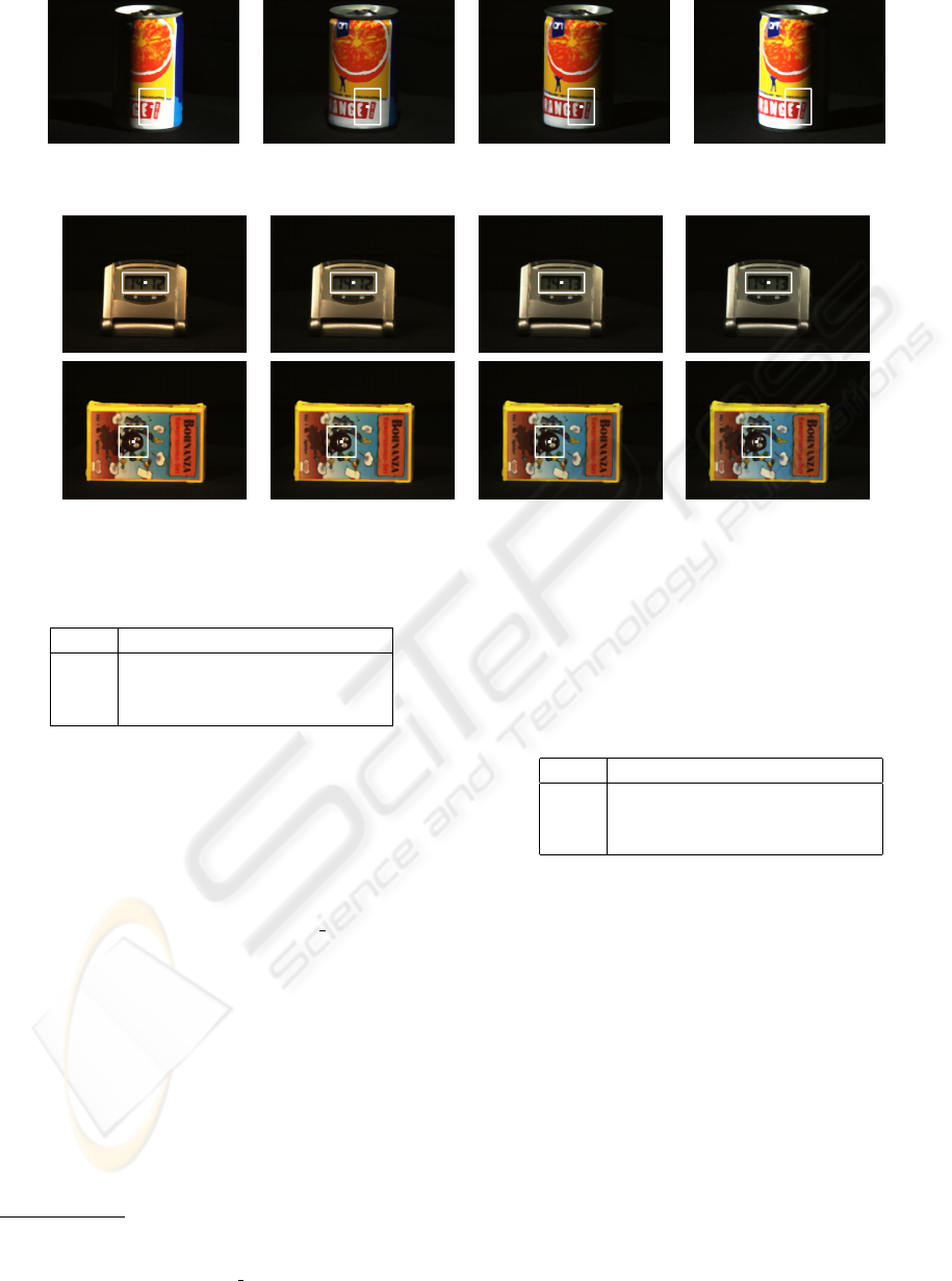
Figure 3: Example of tracking result on the ALOI image data base (object 616) for a change of lighting direction.
Figure 4: Example of tracking result on the ALOI image data base (objects 104 and 101) for a change of illuminant color.
Table 1: Qualitative results when the lighting direction
varies.
Color Nb Q(P
t
) Q(A
x
) Q(A
y
)
RGB 670 1,6 60,7 56,1
IST 1054 1,3 56,2 46,2
TPR 518 2,4 65,7 61,6
4.2 Object Tracking
Our tracking procedure is tested here on two different
road sequences, the first frames of which are shown
on Fig.5 (a) and Fig.6 (b). Only the HSV and TPR
segments are compared, since RGB segments did not
proved to be efficient in previous experiments. The
first image sequence (Fig.5 (a)) dtneu nebel
2
shows
an evolving scene acquired under the fog. The blue
car is selected manually in the 10
t
h frame and has to
be tracked until it goes out of the field of view. Note
that the appearance of the car changes during the se-
quence.
The second image sequence (Fig.6 (a))
3
shows a
walking pedestrian who turns back and moves away
from the camera. The results obtained with HSV seg-
ments are shown on images 5(b) and 6(b). The car
is lost 10 iterations after its detection, and the track-
ing of the pedestrian is not accurate. The results of
2
This sequence has been acquired by the
KOGS/IAKS Universit
¨
at Karlsruhe. It is available on
http://i21www.ira.uka.de/image sequences/
3
LOVe Project: http://love.univ-bpclermont.fr/
the TPR approach are displayed Fig.5 (c) and Fig.6
(c). Obviously, these latter features provide a far bet-
ter matching accuracy, since the car and the pedestrian
are correctly tracked despite changes in appearance.
Table 2: Qualitative results when the color of illuminant is
changed.
Color Nb. Q(P
t
) Q(A
x
) Q(A
y
)
RGB 1067 3,8 62,6 63,6
IST 1159 4,0 66,0 61,0
TPR 795 6,3 75,3 68,0
5 CONCLUSIONS
This article introduces some features - segments -
bound to dichromatic lines. Their stability for fur-
ther use was here tested in a tracking procedure, under
appearance changes and illuminant color variations.
Motion parameters are computed through a common
weighted voting process. The dichromatic segments
provide the highest tracking quality compared to other
segments defined in HSV or RGB spaces. In addition,
a lower number of segments is extracted in TPR. In-
deed, such ”TPR” lines fit the object physical bound-
aries and are less noise-sensitive, while being robust
to lighting changes.
SEGMENTS OF COLOR LINES - A Comparison through a Tracking Procedure
437

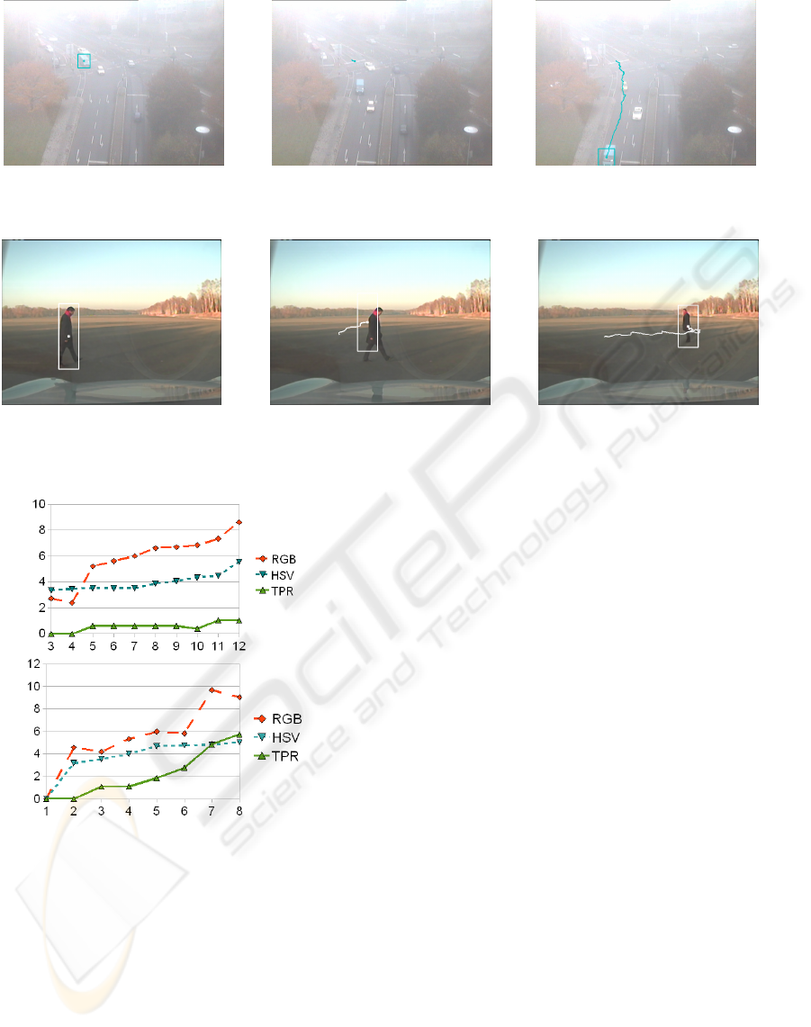
(a) (b) (c)
Figure 5: (a): Initial images with their selected object. (b): Results with HSV segments. (c): Results produced with our
segments.
(a) (b) (c)
Figure 6: (a): Initial images with their selected object. (b): Results with HSV segments. (c): Results produced with our
segments.
(a)
(b)
Figure 7: Evolution of the centroid of the object: (a) for
different colors of illuminant, (b) for different directions of
lighting.
REFERENCES
Baker, S. (2004). Lucas-kanade 20 years on : a unifying
framework. International Journal of Computer Vision,
56(3):221–255.
Bouchafa, S. and Zavidovique, B. (2006). Efficient cumula-
tive matching for image registration. IVC, 24:70–79.
Caselles, V., Coll, B., and Morel, J.-M. (1999). Topo-
graphic maps and local contrast change in natural im-
ages. IJCV, 33(1):5–27.
Caselles, V., Coll, B., and Morel, J.-M. (2002). Geometry
and color in natural images. Journ. of Math. Imag. and
Vis., 16(2):89–105.
Coll, B. and Froment, J. (2000). Topographic maps of color
images. In 15th ICPR, volume 3, pages 613–616.
Comaniciu, D. and Meer, P. (2002). Mean-shift: a robust
approach toward feature space analysis. III Trans. on
PAMI, 24:603–619.
Gevers, T. and Smeulders, A. W. M. (1999). Colour based
object recognition. Pattern Recognition, 32(3):453–
464.
Gouiff
`
es, M. and Zavidovique, B. (2008). A color topo-
graphic map based on the dichromatic model. Eurasip
Journal On IVP.
Hager, G. D. and Belhumeur, P. N. (1998). Efficient region
tracking with parametric models of geometry and illu-
mination. IEEE Trans. on PAMI, 20(10):1025–1039.
Jurie, F. and Dhome, M. (2002). Hyperplane approxima-
tion for template matching. IEEE Trans. on PAMI,
24(7):996–1000.
Lacassagne, L., Manzanera, A., Denoulet, J., and M
´
erigot,
A. (2008). High performance motion detection: Some
trends toward new embedded architectures for vision
systems. Journal of Real Time Image Processing,
DOI10.1007/s11554-008-0096-7.
Paragios, N. and Deriche, R. (2005). Geodesic active re-
gions and level set methods for motion estimation and
tracking. CVIU, 97(3):259–282.
Suvonvorn, N., Coat, F. L., and Zavidovique, B. (2007).
Marrying level-line junctions for obstacle detection.
In IEEE ICIP, pages 305–308.
ICINCO 2009 - 6th International Conference on Informatics in Control, Automation and Robotics
438