
DISTRIBUTED ARRIVAL TIME CONTROL FOR VEHICLE
ROUTING PROBLEMS WITH TIME WINDOWS
Seok Gi Lee and Vittal Prabhu
Harold and Inge Marcus Department of Industrial and Manufacturing Engineering
The Pennsylvania State University, University Park, PA 16802, U.S.A.
Keywords: Distributed Arrival Time Control (DATC), Distributed Control, Scheduling, Dispatching.
Abstract: Competitiveness of a supply chains depends significantly on distribution center operations because it
determines responsiveness and timeliness of deliveries to customers. This paper proposes a control
algorithm for routing multiple out-bound trucks to customers spread over a wide geographical area, each
occupying different volume in a truck, and having a different delivery time-window. Overall operations are
also constrained by geographical locations of the customers in various zones and dissimilar truck capacities.
Performance of the algorithm is tested using data from a distribution center located in Latin America.
1 INTRODUCTION
Transportation is the most expensive logistics
activity. The overall goal in transportation should be
to connect sourcing locations with customers at the
lowest possible transportation cost within the
constraints of the customer service policy (Edward
H. Frazelle, 2002). Most important factors which
can affect transportation cost are the number of
trucks to deliver customer products, shipments
allocation on trucks which decide a route of a truck
and shipments loading on trucks as shown Figure 1.
The truck (vehicle) routing problem has been
recognized for over 40 years and is one of the most
important factors in distribution and logistics. In
particular, the importance of on-time delivery for
customers is growing up according to various and
complicated customer needs. In these conditions,
finding solution optimally is very hard because of
dynamics of a transportation environment. Many
heuristics approach which can be broadly classified
into two main classes, classical heuristics and meta-
heuristics, have been proposed for vehicle routing
problem in a last half century (Gilbert Laporte,
Michel Gendreau, Jean-Yves Potvin, Frederic
Semet, 2000).
Several meta-heuristic methods have been
proposed to solve the vehicle routing problem. The
important issues of meta-heuristics for the vehicle
routing problems is how they can diversify search
space and intensify routing solution to reduce
transportation cost. For example, tabu search and
simulated annealing algorithm tried to jump out of
the local minimum by search its neighborhood
space. To improve limitation of their neighborhood
search space, some advanced methods were
developed and plugged in search logic to diversify
neighborhood search space (Haibing Li, Andrew
Lim, 2003, J-F Cordeau, G Laporte and A Mercier,
2001).
Figure 1: Transportation problem.
Furthermore, research for system dynamism has
been conducted recently. Some measurements were
proposed to explain how dynamic vehicle routing
system (A Larsen, O Madsen and M Solomon, 2002,
Larsen A, 2000). These measurements can play a
crucial role in determining proper models or
algorithms to solve vehicle routing problem
according to the dynamic characteristics of the
system.
246
Gi Lee S. and Prabhu V. (2009).
DISTRIBUTED ARRIVAL TIME CONTROL FOR VEHICLE ROUTING PROBLEMS WITH TIME WINDOWS.
In Proceedings of the 6th International Conference on Informatics in Control, Automation and Robotics - Intelligent Control Systems and Optimization,
pages 246-251
DOI: 10.5220/0002211802460251
Copyright
c
SciTePress
`
In this paper, truck assignment and routing
algorithm (TARA) is proposed to meet not only
transportation cost needs but also customer service
needs. Core of TARA algorithm is constructed based
on distributed arrival time control (DATC) which is
a feedback control-based scheduling approach that
attempts to minimize the average of the square of the
due-date deviation for Just-in-Time system (Hong,
J., Prabhu, V. V., 2003).
2 PROBLEM DEFINETION
The problem, in terms of the distribution center and
customer delivery, could be described as follow. The
distribution center run 24 hours to process
customers’ transportation orders, but trucks operate
loading and control jobs from 4 AM to 10 PM at the
distribution center. During this time, there is no out-
of-order of trucks which is used for delivery. All
trucks are assumed to return to the distribution
center and to be ready for loading at 4 AM.
The problem has three major constraints related
with truck loading, delivery time and order
processing. For truck loading constraints, each truck
has own pallet capacity limit and maximum number
of the customer order in a truck is four. Also, there
are exclusive shipping requests which cannot share
trucks with other shipments. For delivery time
constraints, there are three different types of time
window in this problem. In a sense, a time window
implies the open time of a distribution center. A
customer can request three type of time window. At
first, for specific time of a specific date, delivery
should be as punctual as possible. This is similar to
Just-in-Time strategy with minimizing earliness and
tardiness. Secondly, delivery could be done within a
time window (w
min
, w
max
). Lastly, there could be no
time requirement from customers. It means that a
time window is within (0, 24) hour. Travel time
among each customer’s location including
distribution center is shown in Table 1. For order
processing constraints, customer orders arereceived
every day, except on Sunday, until 6 PM. The
scheduler generates the shipments of the next day. In
other words, every customer order must be shipped
the day after its arrival. Hence, if the distribution
center cannot ship an order due to no available
trucks, the customer order will be shipped the next
earliest truck-available date, which will turn out to
be a large deviation from the requested time
window.
The truck assignment and routing algorithm is
evaluated by two objective functions which are
related with the trucking cost and customer service.
The first objective function for trucking cost can be
determined as follow:
Minimize
11
mm
j
jjj
jj
nC nF
==
⋅
+⋅
∑∑
(1)
where
Sj
∈
∀
, S is the index set of trucks which
are used for delivery, n
j
is the number of trucks type
j, F
j
is the fixed cost for operating one truck and C
j
is the trucking cost of truck type j. The second
objective function related with customer service can
be represented by time window violation cost and
formulated as follow:
Minimize
1
n
i
i
ETC
=
∑
(2)
where ETC
i
= αxmax{0, w
i
min
– c
i
} + βxmax{0, c
i
–
w
i
max
} and c
i
is completion time of customer order i.
In this equation, α is the penalty cost for earliness
and β represents the penalty cost for tardiness of
time window for customer i.
Table 1: Customer location and travel time.
Location
Code
L10001 L10002 L10003 •
L10001 0.00 0.42 0.44 •
L10002 0.42 0.00 0.50 •
L10003 0.44 0.50 0.00 •
L10004 2.05 2.16 1.83 •
L10005 0.75 0.80 0.49 •
L10006 0.84 0.92 0.59 •
• • • • •
3 DISTRIBUTED TIME
CONTROL FOR TRUCK
ASSIGNMENT
DATC is a closed-loop distributed control algorithm
for manufacturing shop floor in which each part
controller uses only its local information to
minimize deviation from its part’s due-date (Hong,
J., Prabhu, V. V., 2003
). In DATC, the integral
control law is represented as follow:
∫
+−=
t
iiiii
adcdkta
0
)0())(()(
ττ
(3)
where k
i
is the controller gain, a
i
(0) is the arbitrary
initial arrival time, d
i
is the due-date and c
i
(τ) is the
predicted completion time for the ith job in the
DISTRIBUTED ARRIVAL TIME CONTROL FOR VEHICLE ROUTING PROBLEMS WITH TIME WINDOWS
247

system. In vehicle routing problem with time
window, the controller gain value is defined by
function of relationship between completion time
and time window and it can be decided according to
two cases, earliness and tardiness. When earliness
occurs, the next arrival time of a job moves toward
minimum value of time window by above integral
control law. Similarly, in case of tardiness, the next
arrival time moves toward maximum value of time
window as shown in Figure 2.
Figure 2: Controller gain adaptation.
The momentum of each arrival time is controlled
by the controller gain, k
i
which is calculated
differently according to the earliness and tardiness as
described in equation (4) and (5).
k
cw
cw
KEk
ii
ii
ii
⋅
−
−
==
min
max
,
min
ii
wc ≤
(4)
k
wc
wc
KTk
ii
ii
ii
⋅
−
−
==
max
min
,
max
ii
wc ≥
(5)
As a result, in case of earliness, equation (3) can
be converted by equation (4) as follow:
)}1({)1()(
min
−−⋅Δ⋅+−= tcwKEtata
iiiii
(6)
Similarly, equation (3) is changed by equation
(5) for the tardiness case as follow:
)}1({)1()(
max
−−⋅Δ⋅+−= tcwKTtata
iiiii
(7)
where a
i
(t) is the arrival time at tth time step, Δ is
the time step and c
i
(t-1) is the completion time at (t-
1)th time step.
Overall TARA procedure is described as follow:
STEP 1 : Initialize customer and truck parameters
a
i
= minimum value of time window – t
1i
c
i
, u
j
= 0, p
j
= P
j
l
j
= 1 (Location 1 implies DC)
STEP 2 : Sort customer based on FCFS rule
STEP 3 : Truck assignment for each customer
For i = 1 to n Do
For j = 1 to m Do
j = Arg(min(E
j
)), subject to v
i
≤ p
j
e
j
= E
j
, p
j
= p
j
– v
i
, l
j
= l
i
u
j
= e
j
+ v
i
/R, where R is the unloading
rate in pallets/hour
c
i
= u
j
a
i
= a
i
+ k
i
x Δ x (d
i
- c
i
)
E
j
= u
j
+ t
ji
STEP 4 : Compute summation of total earliness and
tardiness for each i
STEP 5 : Initialize customer and truck parameters
STEP 6 : Go to STEP 2:
In these TARA steps, a
i
is arrival time of
customer i, c
i
is delivery completion time of
customer i, p
j
is the number of pallets it can be
loaded based on the current load of truck j, p
j
is the
maximum number of pallets it can be loaded by
truck j, l
j
is the current location of the truck j, l
i
is the
location of customer i, u
j
is the last unloading time
of truck j, v
i
is the number of pallet of customer i
and E
j
is time consumption of truck j from current
location to customer i. Also, by equation (6) and (7),
k
i
is KE
i
in case of earliness or KT
i
when the
completion time is greater than maximum value of
time window.
4 TRUCK ASSIGNEMNT AND
ROUTING ALGORITHM
PERFORMANCE
4.1 Performance Comparison
To measure the TARA performance, we used the
following scalar equation (8) for mean squared due
date deviation (MSD) which is used to characterize
the global dynamics (
Prabhu, V. V., 2003).
MSD =
2
1
()
n
ii
i
cd
n
=
−
∑
(8)
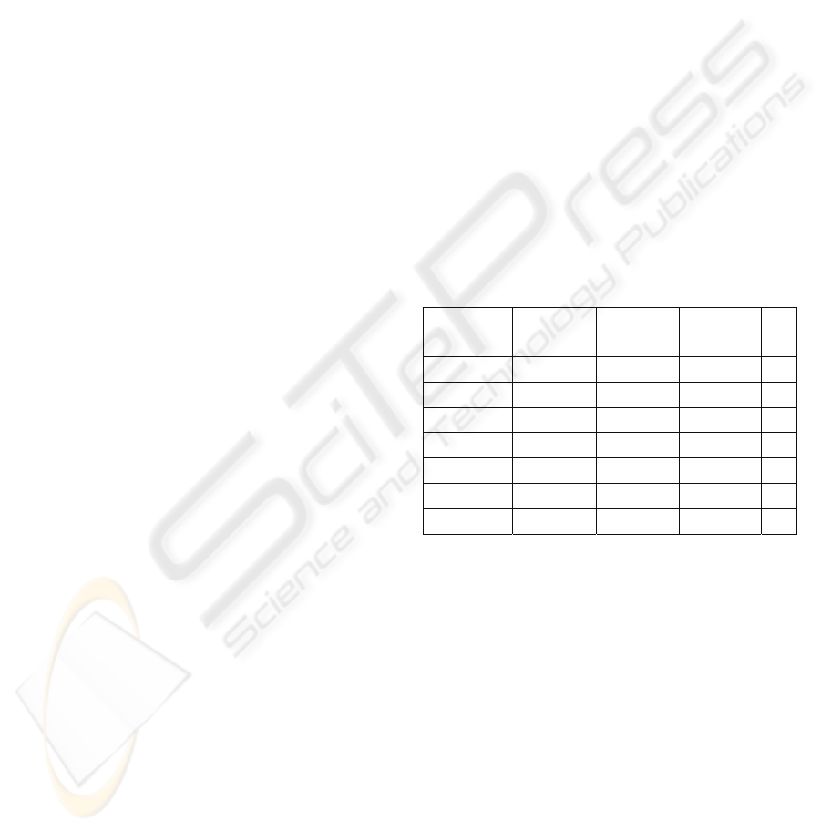
Four customer demand sets which have 24, 31,
43 and 54 orders in them were used for test. These
customer order data were real-world data used by
one of global health and hygiene companies. The
number of trucks was fixed as 12 and they have
equal capacity to load 60 pallets. According to
experiments, in case of set 1, 2 and 4, MSD became
zero within 20th iteration. For set 3, time violation
became the minimum value at 9th iteration. The
MSD results for four kinds of data sets are described
in Figure 3.
Furthermore, by using these experimental data,
TARA performance was compared to dispatch rules,
such as earliest due date (EDD), shortest processing
-
k
+
k
i
a
i
a
max
i
w
min
i
w
ICINCO 2009 - 6th International Conference on Informatics in Control, Automation and Robotics
248
`
time (SPT) and latest processing time (LPT) as
shown in Table 2. For the EDD rule, customer
orders are arranged in ascending order by amount of
time difference between each order’s maximum time
window and distance from the distribution center.
Then each order is loaded in trucks one after another
and finally, total MSD is calculated. For the SPT
rule, orders are arranged in ascending order by
distance between the distribution center and each
order. Then, similar with the EDD rule, each order is
loaded in trucks and total MSD is calculated. In case
of the LPT rule, customer orders are arranged in
descending order by same measurement with the
SPT rule. The number of trucks was fixed as 12.
As a result, for average MSD of four data sets,
TARA obtained 196% better result than the EDD
rule. For the SPT and LPT rules, TARA showed
approximately 199.6% improved results.
Experimental Results of minimum travel
distance for each experiment set are shown in Table
3. Travel distance is estimated by assuming that the
average trucking distance is 60 miles per hour. For
set 1 and set 2 which have relatively small amount
of customer orders, TARA with static controller gain
have same or better performance than dynamic
controller gain. In case of large amount of customer
orders, TARA with dynamic controller gain gives
relatively better performance. However, for almost
all cases, dispatch rules have relatively better
performance than TARA. This is because, basically,
TARA controller proposed in this paper is designed
to minimize tardiness and earliness of customer
orders and it does not contain any device to consider
travel distance.
0
20
40
60
80
100
120
140
160
180
200
1 3 5 7 9 11 13 15 17 19 21 23 25
Ite ration
MSD
Set 1 Set 2 Set 3 Set 4
Figure 3: Mean squared due date deviation.
Table 2: Performance comparison – MSD.
Num
of
Order
TARA
EDD SPT LPT
Static Dynamic
24 0.394 0.000 0.676 5.720 5.367
31 0.000 0.000 0.601 5.636 4.912
43 0.015 0.086 0.544 5.377 4.552
54 0.225 0.000 0.637 5.368 4.153
Table 3: Performance comparison – Travel Distance.
Num
of
Order
TARA
EDD SPT LPT
Static Dynamic
24
1504 1504 1606 1409 1560
31
1635 1749 1861 1591 1905
43
2454 2427 2387 2105 2699
54
2959 2953 3320 2553 2926
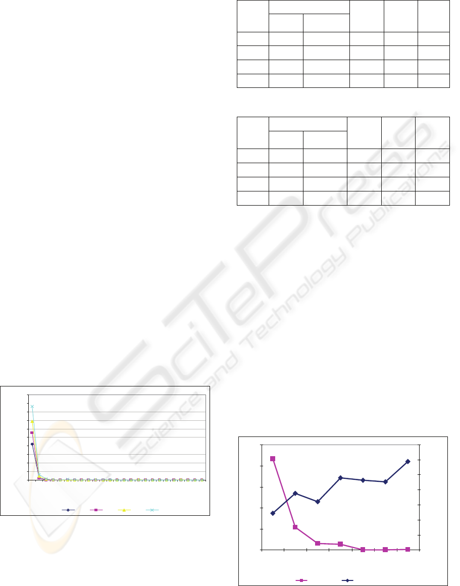
4.2 Trucking Cost
Average total tardiness and average trucking cost
were measured by varying the number of truck for
TARA. To calculate trucking cost, fuel efficiency
was estimated by 15 miles per gallon and fuel price
was assumed by $3.5 per gallon. Also, fixed cost for
a truck which has 1-ton capacity was assumed $0.25
per mile based on the Excel software program
developed by the Texas A&M university (Ron
Torrell, Willie Riggs and Duane Griffith). The
number of customer orders and the controller gain
value was set to 43 and 0.6. Experimental results for
these two measurements are described in Figure 4.
As the number of truck increases, average total
tardiness increases. On the contrary, average
trucking cost decreases as the number of truck
increases.
0
5
10
15
20
25
45678910
Number of Trucks
Time Violation
900
950
1000
1050
1100
1150
1200
1250
Trucking Cost
Tim e V i ol at i on Trucking Cost
Figure 4: Trucking cost & time violation.
DISTRIBUTED ARRIVAL TIME CONTROL FOR VEHICLE ROUTING PROBLEMS WITH TIME WINDOWS
249
0
50
100
150
200
250
45678910
Number of Trucks
Time Violation (Hour)
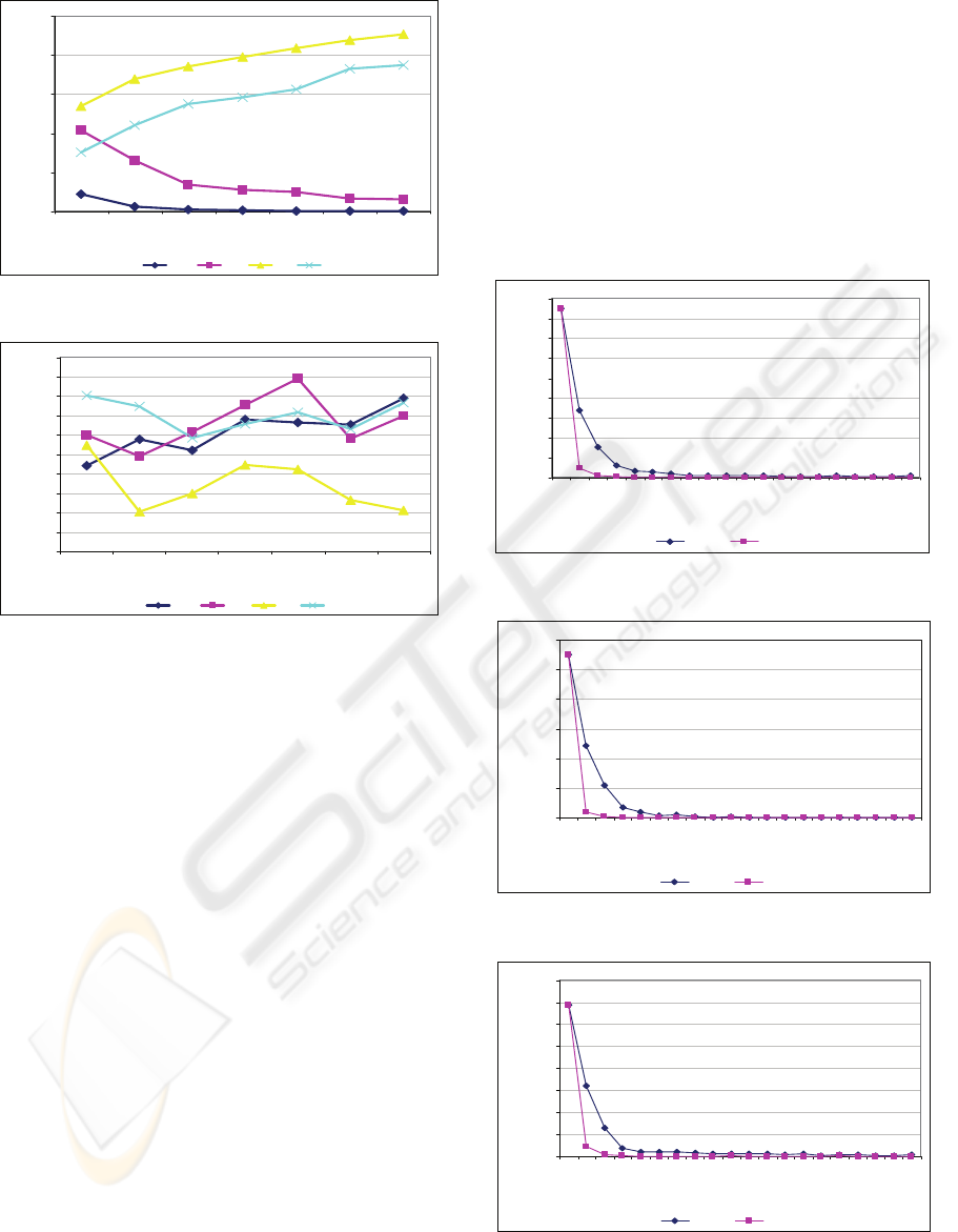
TARA EDD SPT LPT
Figure 5: Time violation comparison.
800
850
900
950
1000
1050
1100
1150
1200
1250
1300
45678910
Number of Trucks
Trucking Cost
TARA EDD SPT LPT
Figure 6: Trucking cost comparison.
Also, time violation and the trucking cost
comparison among TARA and dispatch rules are
shown in Figure 5 and Figure 6. In case of time
violation, TARA and EDD had smaller time
violation value as increasing the number of trucks.
SPT and LPT, however, had increasing time
violation value as increasing the number of trucks.
In case of the trucking cost, it is hard to capture the
relationship between the number of trucks and the
trucking cost as shown Figure 6.
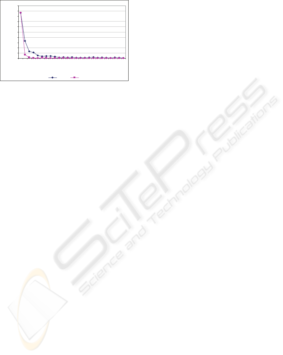
4.2 Dynamic Controller Gain Effects
As we explained in equation (4) and (5), TARA used
dynamic controller gain which is changed by status
of completion time. Actually, the basic distributed
arrival time control updates the arrival time
continuously with the static controller gain through
fixed iteration. However, by changing the controller
gain dynamically according to the status of
completion time, earliness and tardiness, the
convergence velocity and quality of MSD were
improved as shown in Figure 7-10. In case of the 24
orders set (set 1), MSD from the dynamic controller
gain reached zero at 14th iteration, but MSD from
the static controller gain was greater than zero and it
was not converged in zero. Similar results could be
observed in other data sets. For the 31 (set 2), 54 (set
4) order sets, MSD from the dynamic controller gain
were converged in zero at 8th and 21th iteration. In
case of the 31 order set, however, MSD from the
static controller gain was converged at 20th iteration
and the other one was greater than zero and not
converged. Although MSD by the dynamic
controller gain of the 43 order set (set 3) was not
converged, it was less than the result of the static
controller gain and reached at minimum value faster.
0
10
20
30
40
50
60
70
80
90
1 2 3 4 5 6 7 8 9 1011121314151617181920
Ite ration
MSD
Static K Dynamic K
Figure 7: Dynamic controller gain effect – set 1.
0
20
40
60
80
100
120
1 2 3 4 5 6 7 8 9 1011121314151617181920
Iter ation
MSD
Static K Dynamic K
Figure 8: Dynamic controller gain effect – set 2.
0
20
40
60
80
100
120
140
160
1 2 3 4 5 6 7 8 9 1011121314151617181920
Ite ration
MSD
Static K Dynamic K
Figure 9: Dynamic controller gain effect – set 3.
ICINCO 2009 - 6th International Conference on Informatics in Control, Automation and Robotics
250
`
0
20
40
60
80
100
120
140
160
180
200
1 3 5 7 9 11 13 15 17 19 21 23 25
Iteration
MSD
Static K Dynamic K
Figure 10: Dynamic controller gain effect – set 4.
5 CONCLUSIONS
Truck assignment and routing algorithm is an
effective algorithm based on distributed arrival time
control to solve the vehicle routing problem which
has various delivery time windows of customers. In
this work, TARA using the dynamic controller gain
has been developed to determine the best vehicle
routing plan for maximizing customer service level.
Basically, the controller gain used in basic DATC is
maintained static values through the whole
algorithm processes. The dynamic controller gain,
however, is updated continuously through whole
iteration according to the result of the completion
time, earliness and tardiness. Thus, we can improve
not only the convergence velocity of the solution but
also the quality of the solution compared with
dispatch rules simultaneously.
ACKNOWLEDGEMENTS
The research was partially supported by the Marcus
PSU/Technion Exchange Partnership.
REFERENCES
Prabhu, V. V., 2003, Stable Fault Adaptation in
Distributed Control of Heterarchical Manufacturing
Job Shops, IEEE Transaction on Robotics and
Automation
, 19(1), 142-149.
Hong, J., Prabhu, V. V., 2003, Modelling and performance
of distributed algorithm for scheduling dissimilar
machines with set-up,
International Journal of
Production Research
, 41:18, 4357-4382.
Edward H. Frazelle, 2002, Supply Chain Strategy,
McGraw-Hill.
Gilbert Laporte, Michel Gendreau, Jean-Yves Potvin,
Frederic Semet, 2000, Classical and Modern
Heuristics for the Vehicle Routing Problem,
International Transactions in Operational Research,
Res. 7, 285-300.
Haibing Li, Andrew Lim, 2003, Local Search with
annealing-like restarts to solve the VRPTW,
European
Journal of Operational Research
, 150, 115–127.
J-F Cordeau, G Laporte and A Mercier, 2001, A Unified
Tabu Search Heuristic for Vehicle Routing Problems
with Time Windows,
Journal of the Operational
Research Society
, 52, 928-936.
A Larsen, O Madsen and M Solomon, 2002, Partially
Dynamic Vehicle Routing Models and Algorithms,
Journal of the Operational Research Society, 53, 637-
646.
Larsen A, 2000, The dynamic vehicle routing problem,
PhD thesis, Technical University of Denmark.
Ron Torrell, Willie Riggs and Duane Griffith, 2008, Find
out how much truck costs per mile,
www.westernfamerstockman.com.
DISTRIBUTED ARRIVAL TIME CONTROL FOR VEHICLE ROUTING PROBLEMS WITH TIME WINDOWS
251
