A GENERAL MODEL FOR JOB SHOP PROBLEMS USING

IMUNE-GENETIC ALGORITHM AND MULTIOBJECTIVE

OPTIMIZATION TECHNIQUES

Q. Zhang, H. Manier and M.-A. Manier

University of Technology of Belfort-Montbéliard, laboratory Systems and Transport

90010 Belfort Cedex, France

Keywords: Shop scheduling problem with transportation constraints, Immune-genetic algorithm, Multiobjective

optimization, Pareto.

Abstract: We define a global model to simulate the characteristics of three kinds of the manufacturing systems with

transport resources. Based on this model, we use an immune-based genetic algorithm to solve the associated

scheduling problems. We take the makespan and minimum storage as the two objectives and use modified

Pareto ranking method to solve this problem. We show how to choose the best solutions for the studied

systems. Though not all the constraints of the real systems are considered until now, the computational

results show that our proposed model and algorithm have efficiencies in solving scheduling problems.

1 INTRODUCTION

During the past decade, problems in production

planning have been arisen dramatically in automated

manufacturing systems. A well planed

synchronization between the machines and the

transportation resources are crucial to improve their

efficiency. Most of the classical works do not

consider transport operations constraints. However,

material handling systems may become critical

resources. Moreover numerous practical constraints

have to be taken into account, and several objectives

have to be considered. Multiobjective optimization

no doubt plays a very important role to get a more

realistic solution for the decision maker.

In this paper, we consider the manufacturing

systems with transportation resources which can be

classified into mainly three main classes: flexible

manufacturing systems (FMS), robotic cells (RC),

and treatment surface facilities (TSF). A

classification can be found in the literature for each

of these systems (Hall et al., 1998, Tacquard &

Martineau, 2001, Manier & Bloch, 2003, Brauner et

al., 2005). In each system, the associated scheduling

problems can be considered as specific ones.

Nevertheless, there also exist similarities among

them. In fact, there is few works related to the

general problems which link the scheduling of

product operations and transportation together.

Knust (Knust, 1999) integrated the transportation

issues into classical scheduling models. In the same

way, we try to define a global model suitable for any

of those systems with transportation constraints

(section 2). An improved immune-based genetic

algorithm and a modified Pareto-compliant ranking

method are applied as the main solving methods to

solve the scheduling problem with two objectives

(minimization of the makespan and the storage)

(section 3). The computational results for the

proposed algorithm show that our model and the

adopted algorithm are efficient enough to schedule

the activities of production (section 4).

2 GENERAL MODEL

2.1 Notation

Our notations consider the following four aspects:

1) Job/task

n : total number of jobs.

: number of the operations of job i (i ∈[1, n]).

P(i,j): operation j of job i (j ∈[1, O

]).

ijk

: processing time for P(i,j)), on machine MP

−

kij

: minimal processing time of P(i,j) on machine

390

Zhang Q., Manier H. and Manier M. (2009).

A GENERAL MODEL FOR JOB SHOP PROBLEMS USING IMUNE-GENETIC ALGORITHM AND MULTIOBJECTIVE OPTIMIZATION TECHNIQUES.

In Proceedings of the 6th International Conference on Informatics in Control, Automation and Robotics - Intelligent Control Systems and Optimization,

pages 390-393

DOI: 10.5220/0002212303900393

 SciTePress

ijk

: maximal processing time of P(i,j) on machine

: due date of job i, i ∈[1, n].

: starting date of P(i,j). (i ∈[1, n], j ∈[1, O

])

: completion time of job i.

2) Processing Resources

MP: total set of the machines (processing resources)

: machine k (k ∈ [1, ⎜MP⎜]) (unitary capacity).

: is the total set of the processing resources that

can perform operation j of job i . (i ∈[1, n], j ∈[1,

]).

ijk

: PJ

ijk

=1, if the operation j of job i is performed

by machine MP

; PJ

ijk

=0, otherwise

iji’jk

: =1, if P(i, j) is performed right before P(i', j')

on the machine MP

; =0, otherwise

iji’j’k

: setup time on MP

between P(i,j) and P(i’,j’).

3) Transportation Resources

MT: total set of the transportations.

: transportation resource h (Unitary capacity).

T(i, j): transportation task between P(i, j) and P(i,

j+1).

: total set of the transportation resources that can

transport T(i, j).

−

l ,

l : needed time for a transportation resource

to unload (respectively to load) machine MP

kk'h

: empty travel time between machine MP

and

k’

by transportation resource MT

, k, k’ ∈ [1,

|MP|], h∈[1, |MT|].

kk’h

: loaded travel time between machines MP

and

k’

by transportation resource MT

.(it includes

−

and

)

ijh

: =1, if T(i, j) is performed by MT

; =0,

otherwise.

iji’j’h

: =1, if MT

performs T(i, j) right before T(i',

j'); YT

iji’j’h

=0, otherwise.

4) Storage Configuration:

−s

ijk

:time of the input buffer for P(i,j) treated on

ijk

: time of the output buffer for P(i,j) on MP

2.2 Mathematical Model

The objectives of the general model are to minimize

the makespan and the minimal storage:

ijk

PRk

ijkiOii

ntoi

PJptCCMaxCMin

×+==

∑

∈

),(max

)(

∑∑∑

∈∈∈

+−

×+×

MPkniOj

ijkijk

PJPJMin

γγ

And the following constraints of the problem are

respected.

]1,1[],,1[

−

∈

∀

∈

∀

Ojni

PRk

ijkijkij

tPJpt

≤×+

∑

∈

(1)

],1[ ni

∈

∀

],1[

∈

∀

PRk

∈

∀

+−

≤≤

ijkijkijk

Ppp

(2)

],1[ ni

∈

∀

],1[

∈

∀

∑

∈

PRk

ijk

(3)

],1[ ni

∈

∀

]1,1[

−

∈

∀

∑

∈

TRh

ijh

(4)

],1[)',( nii ∈∀

],1[

∈

∀

],1['

Oj ∈

∀

'' jiij

PRPRk

∩

∈

∀

, and M is a very large fixed

number.

MYPtsllpt

kjijijikjijikhkhijkij

×−+≤++++

+−−

）1（

''''''

(5)

(

)

ijkjikhkhkjijikjiijk

sllptPJPJ

''''''''

++++×

+−

MYPt

kjijiij

≤

(6)

],1[)',( nii ∈∀

],1[

∈

∀

],1['

Oj ∈∀

'' jiij

TRTRh

∩

∈

∀

ijk

')1(

+ kji

''''

kji

''')1'('

+ kji

hkkhkk

ijkijkij

''''

στγ

++++

MYTpt

hjiji

kjikjiji

×−+++≤

)1(

''''''''''

(7)

hjiijhkhkhkk

kjikjiji

TJTJIpt

''''''''''''''''''

)( ××++++

στγ

MYTpt

ijhji

ijkijkij

×+++≤

(8)

],1[ ni

∈

∀

1/]1,1[ =

−

∈

∀

ijhi

TJOj

ijk

')1(

+ kji

kijijk

PRkPRk

hkk

ijkijk

PRk

ijkij

PJPJPJpt

ij ijij

∈∈

∈

××++×+

∑

τγ

1,'1'1 +

−

≤++

kij

γγ

(9)

Constraint (1) is the precedence constraints between

two operations of job i; constraint (2) is the

processing time constraints for (i,j) on machine MP

;

Constraint (3) makes sure that one operation can

only be assigned to one machine; constraint (4)

makes sure that one operation can only be assigned

to one transportation resource; constraints (5) and (6)

are the capacity constraints for each processing

resource MP

; constraints (7) and (8) are the

capacity constraints for each transportation resource

; constraint (9) is the travelling constraint, which

expresses that a transportation resource MT

must

have enough time to move a job i between two

successive operations.

A GENERAL MODEL FOR JOB SHOP PROBLEMS USING IMUNE-GENETIC ALGORITHM AND

MULTIOBJECTIVE OPTIMIZATION TECHNIQUES

391

3 RESOLUTION

We use an improved immune-based genetic

algorithm as the training method to find

nondominated solutions of the n-objective

optimization problem.

In our case, we code the antibody into two parts. The

first part is a permutation of the s transportation

tasks (

∑

∈

−=

Os )1(

). The second part is a

permutation of the m operation tasks

(

nsOm

+==

∑

∈

3.1 Selection Operation

In the algorithm (Zhang et al., 2006), the affinity

between antigen and antibody v, is defined by

optax =

, where

opt

is the fitness of antibody v.

The expected selection probability e

of antibody

v is calculated as: e

= ax

where c

is the density

of antibody v. It can be seen from the above equation

that the antibody with both high fitness and low

density would have more chances to survive.

We define that antibody v and antibody w have

the affinity when the following inequality is satisfied

Lwvf <),(

, where

||),(),(

axaxwvdwvf

−

and |ax

-ax

| is the Euclidean distance,

)exp(

TbLL ⋅×=

，

0>b

，and

0>T

is the

number of evolution generations. L is an increasing

function of evolution generations. The antibody’s

diversity and density would be increased efficiently

with the increase of the evolution generations and

that the suppression would be more powerful to

preserve high diversity. So the algorithm would have

strong ability to control the reproducing process.

3.2 Learning Procedure

The whole learning process of the Pareto-

imune-genetic algorithm can be described as follows:

Step 1. Initialization of the Population. All the

gene bits of each antibody in the first generation are

generated randomly within the feasible domain. In

the initialization stage, we calculate the time

windows

],[

+−

ijij

αα

and

],[

+−

ijij

ββ

, which are the

earliest and the latest starting dates of each operation

P(i, j) and T(i, j) respectively. Then, according to all

the constraints, we narrow down the time windows

for all the operations and transportation tasks. Firstly,

we update the earliest starting dates forwardly.

Secondly, we update latest starting dates backwardly.

Step 2. Calculation of the Time Windows. Then

we allocate the tasks on each transport resource by

randomly sequence. We do the same for each

machine according to constraint (1).

After that, we verify all the time windows. If an

individual is not eligible we generate a new one. We

do this until we obtain an eligible individual. The

initial individual is replaced with this new one.

Step 3. Fitness Calculation. We change the

calculation of the new fitness as

follows:

))1(exp(

−

, which makes the value of

the first objective varies according to the rank. And

we take the Pareto ranking method (Goldberg, 1989)

to calculate the rank. In this paper, the two objective

fitness values are defined as the makespan and the

minimum storage.

Step 4. Evolution of the Population. The algorithm

starts with the initial population that is generated

randomly. The reproduction, crossover and mutation

operators are used to produce the filial generation

superior to their parents. Because it has improved

the affinity calculation and makes the threshold

value a dynamic parameter, it has strong ability to

overcome the shortage of the tendency towards local

optimum value and premature. We take the single

point for crossover and the single bit for mutation.

The reproduction operator is based on not only the

fitness but also the density which plays an important

role in diversity maintenance in immune system.

The aforementioned steps are performed repeatedly

until all the training data are trained completely.

4 RESULTS

Here, we take a simple example of five jobs (n=5),

with:

]5,1[

∀

},,{

321

MTMTMTMT =

],1[ ni

∀

],1[

∈

∀

PRk ∈

∀

|]|,1[ MTh ∈∀

|]|,1[' MPk

∈

∀

，

−

ijk

hkkhkk

, and

−

. The colony size is taken from 10 to 100

respectively, the max evolvement generation is

9000, crossover probability is 0.8 and mutation

probability is 0.15. Other parameters are: b=0.01,

=0.8. We run the program for 100 times, we got the

pareto solutions sets, among which the best

makespan is 9 and the minimum storage is 0.

Fig.2 shows results for a population size 100,

ICINCO 2009 - 6th International Conference on Informatics in Control, Automation and Robotics

392

and a evolvement generation 1000. The Pareto

solutions are the rectangular solutions; the others are

the dominated ones. For manufacturing systems that

required no storage (like in the TSF), the solutions

correspond to makespans 12, 13, 14 or 15. For other

systems that allow storage, we obtain solutions with

better makespan. For this example the best

makespan is 9 with storage 1.

Figure 2: A resolution set with the population size 100,

and with the evolvement generation 1000.

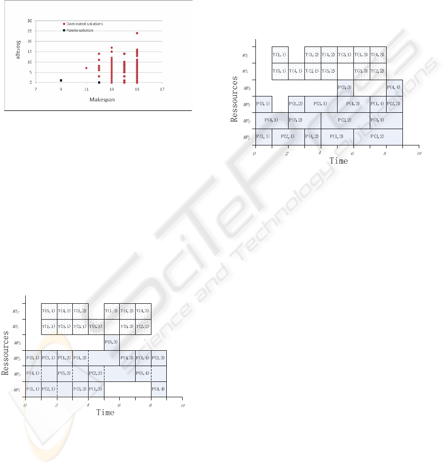
Fig. 3 and 4 respectively present a solution with

and without storage. The dotted (resp. blanked)

squares are transportation tasks (resp. operations);

their width represents the associated times. In Fig. 3,

the dotted line for P(4,2) on MP

means that P(4,2)

can start between time 3 and time 5. The blank

spaces between two transportation tasks represent

the empty movements or waitness of the resource.

The minimum storage corresponds to the time

between T(1,3) and P(1,4) with time windows [6,7].

In Fig. 4, as all the processing times are bounded,

the minimal storage for this solution can reach 0.

Figure 3: The time windows for a solution with makespan

9 and minimal storage 1.

5 CONCLUSIONS

We define a general model which enables us to solve

several kinds of manufacturing schedule problems

with transportation constraints. To reach this goal,

we use pareto-immune-genetic algorithm to schedule

both processing and transport operations. In this

paper, we report our first results for a simplified

model of a production system with or without

storages, and with bounded processing times. In the

future, we will complete this model with the

additional constraints (the configuration of the

transport network and the conflicts between

transport resources). We will also try to improve our

solving algorithm and to compare it with efficient

algorithms developed for each of the considered

systems.

Figure 4: The time windows for a solution with makespan

9 and minimal storage 0.

REFERENCES

Brauner, N., Castagna, P., Espinouse, M., Finke, G.,

Lacomme, P., Martineau, P., Moukrim, A., Soukhal,

A., Tacquard, C. and Tchernev, N., 2005.

Ordonnancement dans les systemes flexibles de

production. RS-JESA, 2005, 39, 925-964.

Goldberg, D. E., 1989. Genetic algorithm in search,

Optimization and machine learning, Addison-Wesley,

Reading, MA, 1989.

Hall, N. G.; Kamounb, H. & Sriskandarajah, C., 1998.

Scheduling in robotic cells: Complexity and steady

state analysis. European Journal of Operational

Research, 1998, 109-1, 43-65.

Knust, S., 1999. Shop-scheduling problems with

transportation. Dissertation, Fachbereich

Mathematik/Informatik, Universität Osnabrück, 1999.

Manier, M.A., Bloch, C, 2003. A Classification for Hoist

Scheduling Problems. The International Journal of

Flexible Manufacturing Systems, 15(2003), 37-55.

Tacquard, C. & Martineau, P., 2001. Automatic notation

of the physical structure of a flexible manufacturing

system. International journal of production economics,

2001, 74, 279-292

Zhang, Q., Xu, X., and Liang, Y.C., 2006. Identification

and speed control of ultrasonic motors based on

modified immune algorithm and Elman neural

networks. Lecture Notes in Artificial Intelligence, Vol.

4259, pp. 746-756, 2006.

A GENERAL MODEL FOR JOB SHOP PROBLEMS USING IMUNE-GENETIC ALGORITHM AND

MULTIOBJECTIVE OPTIMIZATION TECHNIQUES

393