ON MODIFICATION OF THE GENERALISED CONDITIONING
TECHNIQUE ANTI-WINDUP COMPENSATOR
Dariusz Horla
Poznan Univeristy of Technology, Institute of Control and Information Engineering, ul. Piotrowo 3a, 60-965 Poznan, Poland
Keywords:
Back-calculation, Generalised conditioning technique, Anti-windup compensator, Constraints.
Abstract:
New anti-windup scheme is presented in application to pole-placement control, with a complete analysis of
its behaviour for a class of second-order minimumphase stable plants of oscillatory and aperiodic character-
istics with different dead-times. The classical generalised conditioning technique anti-windup compensator
performance is compared with its three proposed modifications, arising in a new GCT compensation scheme.
A critical discussion of the necessity of compensation is also given.
1 INTRODUCTION
Constraints are ubiquitous in real-world environment.
As the result of their presence or the presence of
some nonlinearities in the control loops, arises the
difference in between computed and applied (i.e. con-
strained) control signal. In such a case, the perfor-
mance of the closed-loop system degrades in com-
parison with the performance of the linear system,
when constraints are not active. Such a degradation
is defined as windup phenomenon (Rundqwist, 1991;
Walgama and Sternby, 1990; Walgama and Sternby,
1993).
This can be also viewed from the point of discrep-
ancy in between internal controller states and its out-
put. When there is no correspondence in between
controller’s output and its internal controller states,
the controller does not have any information what the
current value of the constrained control signal is, and
windup phenomenon arises.
The windup phenomenon has been, at first, de-
fined for controllers comprising integral terms, as the
so-called integrator windup (Rundqwist, 1991). For
such controllers, control constraints may cause ex-
cessive integration of the error signal, giving rise to
longer settling of the output signal and overshoots.
There are two strands in compensating windup phe-
nomenon (in AWC, anti-windup compensation) – tak-
ing constraints into account during the design proce-
dure of the controller or assuming the system is linear,
designing the controller for the linear case, and, sub-
sequently, imposing constraints and applying AWCs
(Horla, 2007; Horla and Krolikowski, 2003a; Horla
and Krolikowski, 2003b).
The simplest anti-windup compensatorshave been
based on the idea of integrator clamping, i.e. they
referred to the controllers comprising integral terms
only (Visioli, 2003). The proposed AWCs avoided
integration of the error signal whenever some condi-
tions were met, e.g., the control signal saturated, or
error exceeded some predefined threshold, etc.
Such an approach was simple enough to be easily
implemented, but as it has been already said, applica-
ble to some controllers only.
The advanced anti-windup compensators have
been designed for the case of general controller,
which input-output equation is written in the RST
form. Among the proposed AWCs one can find in the
literature deadbeat, generalised, conditioning tech-
nique, modified conditioning technique and gener-
alised conditioning technique anti-windup compen-
sators (Horla and Krolikowski, 2003a; Horla and Kro-
likowski, 2003b). The three latter AWCs are based on
the idea of back-calculation, i.e. modification of the
signal that the output signal of the plant is to track,
with respect to current saturation level.
The paper focuses on the generalised conditioning
technique AWC (GCT-AWC), being a compromise
solution in between the simplicity of the advanced
AWC and compensation capabilities of the condition-
ing algorithm, what will be explained later.
The main idea of the paper is to present a modifi-
cation of the GCT-AWC that can arise from the idea of
integrator clamping methods, and to show that it can
result in better control performance than performance
33
Horla D. (2009).
ON MODIFICATION OF THE GENERALISED CONDITIONING TECHNIQUE ANTI-WINDUP COMPENSATOR.
In Proceedings of the 6th International Conference on Informatics in Control, Automation and Robotics - Signal Processing, Systems Modeling and
Control, pages 33-38
DOI: 10.5220/0002212700330038
Copyright
c
 SciTePress

of the system with original GCT-AWC. The presented
results refer to the research carried for a set of stable
minimumphase second-order discrete-time plants and
different constraint levels.
There are no remarks in the literature how to
improve the performance of the GCT-AWC, apart
from (Horla and Krolikowski, 2003a). The proposed
method limits the number of modifications, with the
same excess. By introducing the proposed modifica-
tions one can improve the performance of the most
appealing AWC technique.
2 PLANT MODEL
Let the discrete-time CARMA model be given
A(q
−1
)y
t
= B(q
−1
)u
t−d
, (1)
where y
t
is the plant output, u
t
is the constrained con-
trol input, d ≥ 1 is a dead-time and:
A(q
−1
) = 1+ a
1
q
−1
+ a
2
q
−2
, (2)
B(q
−1
) = b
0
+ b
1
q
−1
(3)
are relatively prime. The control signal u
t
= sat(v
t
;α)
is the computed control signal after saturation by
symmetrical cut-off function at level ±α.
3 CONTROLLER
The plant is controlled by the pole-placement con-
troller that ensures tracking of a given reference signal
r
t
by the plant output y
t
with given dynamics,
v
t
= k
R
r
t
− k
P
y
t
+ k
I
q
−1
1− q
−1
(r
t
− y
t
) −
−k
D
1− q
−1
1− γq
−1
y
t
, (4)
where k
R
= rk
P
, r > 0. The above controller equa-
tion can be obtained by discretisation of a continuous-
time PID controller (Rundqwist, 1991), and it can
be rewritten into the RST structure (Horla and Kro-
likowski, 2003b)
R(q
−1
)v
t
= −S(q
−1
)y
t
+ T(q
−1
)r
t
. (5)
Coefficients of polynomials R(q
−1
), S(q
−1
), T(q
−1
)
can be determined by solving the following Diophan-
tine equation
A(q
−1
)R(q
−1
) + q
−d
B(q
−1
)S(q
−1
) =
= A
M
(q
−1
)A
o
(q
−1
), (6)
where polynomials A
o
(q
−1
) and A
M
(q
−1
) are stable,
and given polynomial A
M
(q
−1
) is of second order in
the chapter.
Controller polynomials R(q
−1
), S(q
−1
), T(q
−1
)
are of order d + nB, nA, nA
o
, respectively, and have
forms as follows:
R(q
−1
) = (1− q
−1
)R
′
(q
−1
),
S(q
−1
) = s
0
+ s
1
q
−1
+ s
2
q
−2
, (7)
T(q
−1
) = k
R
A
o
(q
−1
).
From the controller equation (5), given structure
R(q
−1
), S(q
−1
), T(q
−1
) (7) and (4) it follows that:
s
0
= k
P
+ k
D
,
s
1
= k
I
− 2k
D
− k
P
(1+ γ), (8)
s
2
= k
D
− γ(k
I
− k
P
),
A
o
(q
−1
) =

1−γq
−1


1−q
−1

1−
k
I
k
R

=
= 1+ a
o1
q
−1
+ a
o2
q
−2
, (9)
where γ = −
b
1
b
0
, k
R
= rk
P
, a
o1
=
k
I
k
R
− (1 + γ), a
o2
=
γ

1−
k
I
k
R

. As the polynomial A
o
(q
−1
) has to be sta-
ble, 0 <
k
I
k
R
< 2 must hold what can be ensured by
a proper choice of r.
The controller algorithm is assumed to be altered
by anti-windup compensator presented in the next
Section, in order to assure better control performance
of the closed-loop system subject to constraints. It is
to be borne in mind that the compensation is based on
back-calculation, i.e., it does not require the controller
to have integral terms in general.
4 GENERALISED
CONDITIONING TECHNIQUE
AWC
In GCT, the filtered set-point signal is conditioned,
instead of the set-point r
t
, and given as
r
f,t
=
Q(q
−1
)T
1
(q
−1
)
L(q
−1
)
r
t
, (10)
with
T(q
−1
) = T
2
(q
−1
)T
1
(q
−1
),
Q(q
−1
) = q
0
+ q
1
q
−1
+ ··· + q
nQ
q
−nQ
, (11)
L(q
−1
) = 1+ l
1
q
−1
+ ··· + l
nL
q
−nL
and T
2
(0) = t
2,0
.
Similarly to the conditioning method (see (Horla
and Krolikowski, 2003a)), the modified filtered refer-
ence signal is given by
r
r
f,t
= r
f,t
+
q
0
(u
t
− v
t
)
t
2,0
, (12)
ICINCO 2009 - 6th International Conference on Informatics in Control, Automation and Robotics
34

and the control signal is defined as
v
t
= (1− Q
′
(q
−1
)R(q
−1
))u
t
+
t
2,0
q
0
r
f,t
+
+
1
q
0
((T
2
(q
−1
)L(q
−1
) −t
2,0
)r
r
f,t
−
−Q
′
(q
−1
)S(q
−1
)y
t
, (13)
where Q
′
(q
−1
) =
Q(q
−1
)
q
0
.
The GCT method enables additional tuning of the
performance by reference signal filter design. Be-
cause its parameters should correspond to model pa-
rameters, saturation level and set-point values, a spe-
cial choice of parameters of the filter (10) for min-
imumphase second-order model is proposed (Horla
and Krolikowski, 2003a). Let ρ
1
and ρ
2
denote poles
of stable A(z
−1
), then
ρ = max(|ρ
1
|, |ρ
2
|), (14)
Q(q
−1
) = 1+

(1− ρ)
ξ
− 1

q
−1
, (15)
L(q
−1
) = 1− (1− ρ)
ξ
q
−1
, (16)
where 0 < ξ ≤ 1 is the damping factor obtained from
classical root locus theory for the second-order sys-
tems. The suggested filter (14–16) takes into consid-
eration model parameters and set-point values only,
forcing the initial values of the filtered reference sig-
nal for slow models and reducing the amplitude and
rate of transients for oscillatory ones.
The inherent property of the conditioning tech-
nique is the so-called short sightedness phenomenon,
resulting in consecutive resaturations of the control
signal because of excessive modification of the refer-
ence signal. In order to improve the performance of
the compensation three modifications will be consid-
ered as in the next Section.
5 MODIFIED GENERALISED
CONDITIONING AWCS
In order to combine classical conditional integration
methods that work for controllers comprising inte-
grators with back-calculation AWC presented in the
previous Section, the followingthree back-calculation
modifications have been proposed – the modification
of the filtered reference input is applied when:
M1 |e
t
| > e
1
,
M2 u
t−1
6= v
t−1
,
M3 u
t−1
6= v
t−1
and e
t
u
t−1
> 0,
where e
1
is a threshold value for reference modifica-
tion clamping.
By applying the modifications to the GCT-AWC
one assures that modification of the filtered reference
signal is performed only when necessary.
6 SIMULATED PLANTS
The simulations have been performed for a set
of stable, second-order, minimumphase plants with
B(q
−1
) = 1 + 0.5q
−1
and:
• P1 type
A(q
−1
) = (1 − q
−1
(σ+ ωi))(1− q
−1
(σ− ωi)),
where:
−1 < σ < 1,
−1 < ω < 1,
|σ± ωi| < 1,
what corresponds to oscillatory behaviour of the
plant,
• P2 type
A(q
−1
) = (1 − q
−1
z
1
)(1− q
−1
z
2
),
where:
0 < z
1
< 1,
0 < z
2
< 1,
what corresponds to aperiodic behaviour of the
plant.
The simulations have been run for square wave ref-
erence signal of period 40 samples and symmetrical
amplitude ±3 with
k
I
k
R
= 0.5, A
M
(q
−1
) = 1−0.5q
−1
+
0.06q
−2
and e
1
= 3.
In order to evaluate the quality of regulation pro-
cess, the performance index is introduced
J =
1
N
∑
N
t=0
(r
t
− y
t
)
2
, (17)
where N = 150 denotes the simulation horizon.
The simulations have been performed for the same
constraint hardness for each of the plants, denoted by
relative constraint level α
r
(i.e., the multiplicity of
the minimum constraint level α
min
= 3
|A(1)|
|B(1)|
allow-
ing asymptotic tracking). The absolute value of the
constraint is α = α
r
α
min
and changes as the plants
change.
7 PERFORMANCE SURFACES
The results of the simulation tests are shown as per-
formance surfaces. Each of the axes has been divided
into 101 values, thus all simulation results refer to a
grid of 101 × 101 different plants. The idea of such
surfaces is as follows – let J
0
denote the value of the
performance index of the control system with some
plant and given α
r
and no AWC. Let J
1
denote the
value of the performance index of the same control
ON MODIFICATION OF THE GENERALISED CONDITIONING TECHNIQUE ANTI-WINDUP COMPENSATOR
35

system with the same plant but with classical GCT-
AWC. Let J
2
denote the value of the performance in-
dex of, again, the same control system with the same
plant but with modified GCT-AWC (M1, M2 or M3).
For each of the plants and constraints level the fol-
lowing face is plotted:
 (magenta) J
0
= J
1
= J
2
,
 (red) modification is of the worst performance,
J
0
< J
1
< J
2
or J
1
< J
0
< J
2
, the intensity of the
red level is proportional to J
2
− J
0
or J
2
− J
1
,
 (white) modification improves the performance of
the GCT-AWC, J
0
< J
2
< J
1
,
 (black) it is not worth to modify GCT, J
1
< J
2
<
J
0
, the intensity of the black level is proportional
to J
2
− J
1
,
 (blue) modification improves the performance
where GCT fails to, J
2
< J
0
< J
1
, the intensity of
the blue level is proportional to J
0
− J
2
,
 (green) modification is of the best performance,
the intensity of the green level is proportional to
J
0
− J
2
or J
1
− J
2
.
8 SHOULD ONE MODIFY GCT?
The performance surfaces have been obtained for P1
and P2 type plants with different dead-times and pre-
sented in Figs 1 and 2, where consecutive rows for
different dead-times refer to M1, M2 and M3.
In all the cases of P1 and d = 1 it is visible that
all modifications can improve the performance of the
GCT for slow plants, i.e., with small natural fre-
quency, whereas in the case of M1 and M3 there is
an improvement visible for such plants near stability
border. In the case of M1 and M3, one can see re-
gion of the best improvement (green). By comparing
the given surfaces one can say that M3 is of the best
AWC performance, because of the green regions and
brighter red regions than in other cases, what refers to
less performance degradation.
It is not advisable to modify the GCT algorithm
when the region is red, it is advisable to improve
where it is white and definitely advisable when green.
In the case of d = 3 one can see that red regions
have almost disappeared and the improvement is best
in the case of M3.
For P2 type plants a performance improvement
can be observed for slow plants (green) with M1 and
M3. Because of the size of white and green regions
one can say that the best performance is assured by
M1, mainly because of the α
r
> 1, that is visibility of
green regions for greater α
r
s. The vast areas of red
color suggest that it is inadvisable to modify the orig-
inal GCT when plant is moderately slow (expressed
by absolute values of its poles).
In the case of d = 3 because of the area of white
region and brightness of the red region, it can be said
that M1 is the best choice, then M2 and M3.
9 SUMMARY
It has been shown that it can be advantageous to mod-
ify the algorithm of well-known GCT-AWC in order
to obtain high control performance. Such a modifica-
tion can be implemented with the use of lookup table,
where the information is stored what GCT algorithm
should be used when plant parameters vary in time,
e.g. due to aging or set-point change. A similar ap-
proach has been presented for continuoussystem, PID
controllers and integrator clamping (Visioli, 2003).
REFERENCES
Horla, D. (2007). Simple anti-integrator windup compen-
sators – performance analysis. Studies in Control and
Computer Science, 32:85–102.
Horla, D. and Krolikowski, A. (2003a). Anti-windup cir-
cuits in adaptive pole-placement control. In Proceed-
ings of the 7th European Control Conference.
Horla, D. and Krolikowski, A. (2003b). Anti-windup com-
pensators for adaptive pid controllers. In Proceedings
of the 9th IEEE International Conference on Methods
and Models in Automation and Robotics, pages 575–
580.
Rundqwist, L. (1991). Anti-reset Windup for PID Con-
trollers. PhD thesis, Lund University of Technology.
Visioli, A. (2003). Modified anti-windup scheme for pid
controllers. IEE Proceedings-D, 150(1):49–54.
Walgama, K. and Sternby, J. (1990). Inherent observer
property in a class of anti-windup compensators. In-
ternational Journal of Control, 52(3):705–724.
Walgama, K. and Sternby, J. (1993). On the convergence
properties of adaptive pole-placement controllers with
anti-windup compensators. IEEE Transactions on Au-
tomatic Control, 38(1):128–132.
ICINCO 2009 - 6th International Conference on Informatics in Control, Automation and Robotics
36

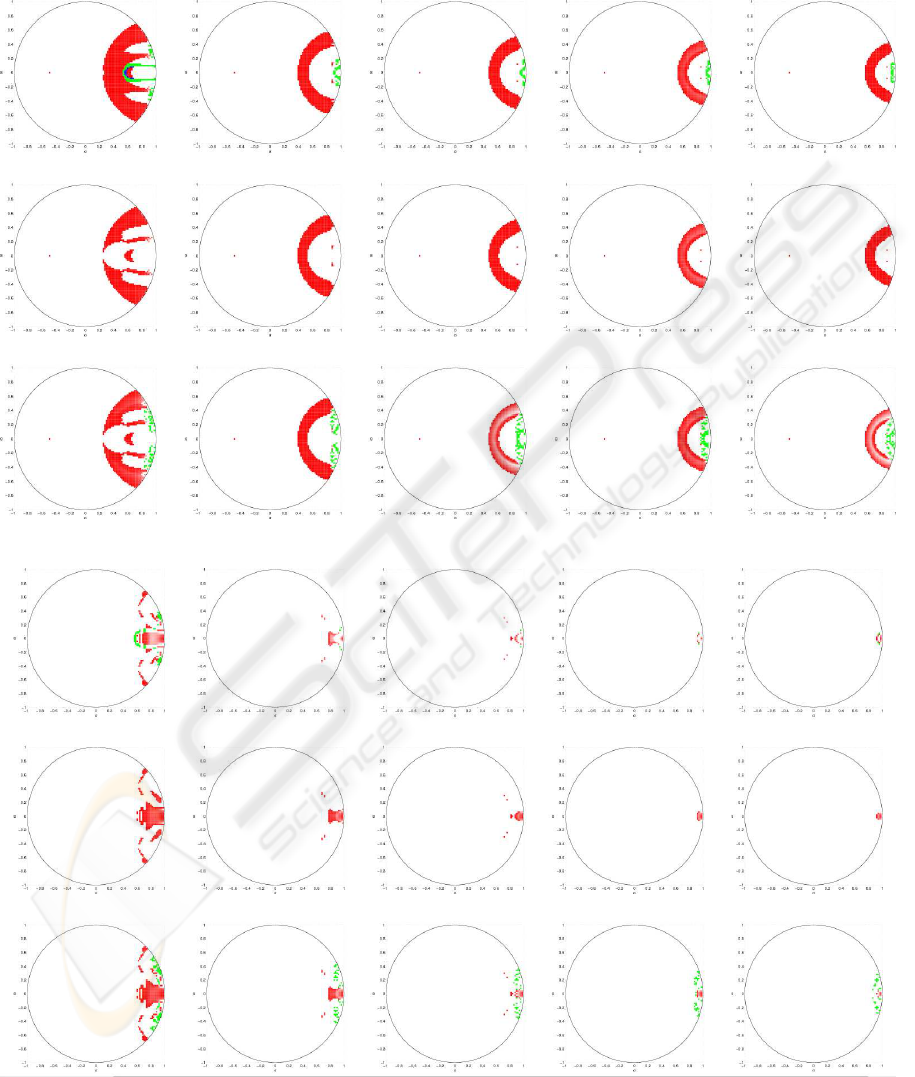
α
r
= 1 α
r
= 2 α
r
= 3 α
r
= 4 α
r
= 5
d = 1
d = 3
Figure 1: Performance surfaces for P1.
ON MODIFICATION OF THE GENERALISED CONDITIONING TECHNIQUE ANTI-WINDUP COMPENSATOR
37

α
r
= 1 α
r
= 2 α
r
= 3 α
r
= 4 α
r
= 5
d = 1
d = 3
Figure 2: Performance surfaces for P2.
ICINCO 2009 - 6th International Conference on Informatics in Control, Automation and Robotics
38