
VISION-BASED AUTONOMOUS APPROACH AND LANDING FOR
AN AIRCRAFT USING A DIRECT VISUAL TRACKING METHOD
Tiago F. Gonc¸alves, Jos´e R. Azinheira
IDMEC, IST/TULisbon, Av. Rovisco Pais N.1, 1049-001 Lisboa, Portugal
Patrick Rives
INRIA-Sophia Antipolis, 2004 Route des Lucioles, BP93, 06902 Sophia-Antipolis, France
Keywords:
Aircraft autonomous approach and landing, Vision-based control, Linear optimal control, Dense visual track-
ing.
Abstract:
This paper presents a feasibility study of a vision-based autonomous approach and landing for an aircraft using
a direct visual tracking method. Auto-landing systems based on the Instrument Landing System (ILS) have
already proven their importance through decades but general aviation stills without cost-effective solutions
for such conditions. However, vision-based systems have shown to have the adequate characteristics for the
positioning relatively to the landing runway. In the present paper, rather than points, lines or other features
susceptible of extraction and matching errors, dense information is tracked in the sequence of captured images
using an Efficient Second-Order Minimization (ESM) method. Robust under arbitrary illumination changes
and with real-time capability, the proposed visual tracker suits all conditions to use images from standard
CCD/CMOS to Infrared (IR) and radar imagery sensors. An optimal control design is then proposed using the
homography matrix as visual information in two distinct approaches: reconstructing the position and attitude
(pose) of the aircraft from the visual signals and applying the visual signals directly into the control loop. To
demonstrate the proposed concept, simulation results under realistic atmospheric disturbances are presented.
1 INTRODUCTION
Approach and landing are known to be the most de-
manding flight phase in fixed-wing flight operations.
Due to the altitudes involved in flight and the con-
sequent nonexisting depth perception, pilots must in-
terpret position, attitude and distance to the runway
using only two-dimensional cues like perspective, an-
gular size and movement of the runway. At the same
time, all six degrees of freedom of the aircraft must be
controlled and coordinated in order to meet and track
the correct glidepath till the touchdown.
In poor visibility conditions and degraded visual
references, landing aids must be considered. The In-
strument Landing System (ILS) is widely used in most
of the international airports around the world allow-
ing pilots to establish on the approach and follow the
ILS, in autopilot or not, until the decision height is
reached. At this point, the pilot must have visual con-
tact with the runway to continue the approach and
proceed to the flare manoeuvre or, if it is not the
case, to abort. This procedure has proven its relia-
bility through decades but landing aids systems that
require onboard equipment are still not cost-effective
for most of the general airports. However, in the
last years, the Enhanced Visual Systems (EVS) based
on Infrared (IR) allowed the capability to proceed to
non-precision approaches and obstacle detection for
all weather conditions. The vision-based control sys-
tem proposed in the present paper intends then to take
advantage of these emergent vision sensors in order to
allow precision approaches and autonomous landing.
The intention of using vision systems for au-
tonomous landings or simply estimate the aircraft po-
sition and attitude (pose) is not new. Flight tests of
a vision-based autonomous landing relying on fea-
ture points on the runway were already referred by
(Dickmanns and Schell, 1992) whilst (Chatterji et al.,
1998) present a feasibility study on pose determina-
tion for an aircraft night landing based on a model
of the Approach Lighting System (ALS). Many oth-
ers have followed in using vision-based control on
94
F. Gonçalves T., R. Azinheira J. and Rives P. (2009).
VISION-BASED AUTONOMOUS APPROACH AND LANDING FOR AN AIRCRAFT USING A DIRECT VISUAL TRACKING METHOD.
In Proceedings of the 6th International Conference on Informatics in Control, Automation and Robotics - Robotics and Automation, pages 94-101
DOI: 10.5220/0002212900940101
Copyright
c
SciTePress

fixed/rotary wings aircrafts, and even airships, in sev-
eral goals since autonomous aerial refueling ((Kim-
mett et al., 2002), (Mati et al., 2006)), stabiliza-
tion with respect to a target ((Hamel and Mahony,
2002), (Azinheira et al., 2002)), linear structures
following ((Silveira et al., 2003), (Rives and Azin-
heira, 2004), (Mahony and Hamel, 2005)) and, obvi-
ously, automatic landing ((Sharp et al., 2002), (Rives
and Azinheira, 2002), (Proctor and Johnson, 2004),
(Bourquardez and Chaumette, 2007a), (Bourquardez
and Chaumette, 2007b)). In these problems, differ-
ent types of visual features were considered including
geometric model of the target, points, corners of the
runway, binormalized Plucker coordinates, the three
parallel lines of the runway (at left, center and right
sides) and the two parallel lines of the runway along
with the horizon line and the vanishing point. Due to
the standard geometry of the landing runway and the
decoupling capabilities, the last two approaches have
been preferred in problems of autonomous landing.
In contrast with feature extraction methods, direct
or dense methods are known by their accuracy be-
cause all the information in the image is used with-
out intermediate processes, reducing then the sources
of errors. The usual disadvantage of such method is
the computational consuming of the sum-of-squared-
differences minimization due to the computation of
the Hessian matrix. The Efficient Second-order Mini-
mization (ESM) (Malis, 2004) (Behimane and Malis,
2004) (Malis, 2007) method does not require the
computation of the Hessian matrix maintaining how-
ever the high convergence rate characteristic of the
second-order minimizations as the Newton method.
Robust under arbitrary illumination changes (Silveira
and Malis, 2007) and with real-time capability, the
ESM suits all the requirements to use images from
the common CCD/CMOS to IR sensors.
In vision-based or visual servoing problems, a pla-
nar scene plays an important role since it simplifies
the computation of the projective transformation be-
tween two images of the scene: the planar homogra-
phy. The Euclidean homography, computed with the
knowledge of the calibration matrix of the imagery
sensor, is here considered as the visual signal to use
into the control loop in two distinct schemes. The
position-based visual servoing (PBVS) uses the re-
covered pose of the aircraft from the estimated projec-
tive transformation whilst the image-based visual ser-
voing (IBVS) uses the visual signal directly into the
control loop by means of the interaction matrix. The
controller gains, from standard output error LQR de-
sign with a PI structure, are common for both schemes
whose results will be then compared with a sensor-
based scheme where precise measures are considered.
The present paper is organized as follows: In the
Section 2, some useful notations in computer vision
are presented, using as example the rigid-body motion
equation, along with an introduction of the consid-
ered frames and a description of the aircraft dynamics
and the pinhole camera models. In the same section,
the two-view geometry is introduced as the basis for
the IBVS control law. The PBVS and IBVS control
laws are then presented in the Section 3 as well as the
optimal controller design. The results are shown in
Section 4 while the final conclusions are presented in
Section 5.
2 THEORETICAL BACKGROUND
2.1 Notations
The rigid-body motion of the frame b with respect to
frame a by
a
R
b
∈ SO(3) and
a
t
b
∈ R
3
, the rotation
matrix and the translation vector respectively, can be
expressed as
a
X =
a
R
b
b
X+
a
t
b
(1)
where,
a
X ∈ R
3
denotes the coordinates of a 3D point
in the frame a or, in a similar manner,in homogeneous
coordinates as
a
X =
a
T
b
b
X =
a
R
b
a
t
b
0 1
b
X
1
(2)
where,
a
T
b
∈ SE(3), 0 denotes a matrix of zeros with
the appropriate dimensions and
a
X ∈ R
4
are the ho-
mogeneous coordinates of the point
a
X. In the same
way, the Coriolis theorem applied to 3D points can
also be expressed in homogenous coordinates, as a re-
sult of the derivative of the rigid-body motion relation
in Eq. (2),
a
˙
X =
a
˙
T
b
b
X =
a
˙
T
b
a
T
−1
b
a
X = (3)
=
b
ω v
0 0
a
X =
a
b
V
ab
a
X ,
a
b
V
ab
∈ R
4×4
where, the angular velocity tensor
b
ω ∈ R
3×3
is the
skew-symmetric matrix of the angular velocity vec-
tor ω such that ω × X =
b
ωX and the vector
a
V
ab
=
[v,ω]
⊤
∈ R
6
denotes the velocity screw and indicates
the velocity of the frame b moving relative to a and
viewed from the frame a. Also important in the
present paper is the definition of stacked matrix, de-
noted by the superscript ”
s
”, where each column is
rearranged into a single column vector.
2.2 Aircraft Dynamic Model
Let F
0
be the earth frame, also called NED for North-
East-Down, whose origin coincides with the desirable
VISION-BASED AUTONOMOUS APPROACH AND LANDING FOR AN AIRCRAFT USING A DIRECT VISUAL
TRACKING METHOD
95

touchdown point in the runway. The latter, unless ex-
plicitly indicated and without loss of generality, will
be considered aligned with North. The aircraft lin-
ear velocity v = [u, v, w] ∈ R
3
, as well as its angular
velocity ω = [p,q,r] ∈ R
3
, is expressed in the air-
craft body frame F
c
whose origin is at the center of
gravity where u is defined towards the aircraft nose,
v towards the right wing and w downwards. The at-
titude, or orientation, of the aircraft with respect to
the earth frame F
0
is stated in terms of Euler angles
Φ = [φ,θ,ψ] ⊂ R
2
, the roll, pitch and yaw angles re-
spectively.
The aircraft motion in atmospheric flight is usu-
ally deduced using Newton’s second law and con-
sidering the motion of the aircraft in the earth frame
F
0
, assumed as an inertial frame, under the influence
of forces and torques due to gravity, propulsion and
aerodynamics. As mentioned above, both linear and
angular velocities of the aircraft are expressed in the
body frame F
b
as well asfor the considered forces and
moments. As a consequence, the Coriolis theorem
must be invoked and the kinematic equations appear
naturally relating the angular velocity rate ω with the
time derivative of the Euler angles
˙
Φ = R
−1
ω and the
instantaneous linear velocity v with the time deriva-
tive of the NED position
˙
N,
˙
E,
˙
D
⊤
= S
⊤
v.
In order to simplify the controller design, it is
common to linearize the non-linear model around an
given equilibrium flight condition, usually a func-
tion of airspeed V
0
and altitude h
0
. This equilib-
rium or trim flight is frequently chosen to be a steady
wings-level flight, without presence of wind distur-
bances, also justified here since non-straight landing
approaches are not considered in the present paper.
The resultant linear model is then function of the per-
turbation in the state vector x and in the input vector
u as
˙x
v
˙x
h
=
A
v
0
0 A
h
x
v
x
h
+
B
v
B
h
u
v
u
h
(4)
describing the dynamics of the two resultant decou-
pled, lateral and longitudinal, motions. The longitu-
dinal, or vertical, state vector is x
v
= [u, w,q,θ]
⊤
∈ R
4
and the respective input vector u
v
= [δ
E
,δ
T
]
⊤
∈ R
2
(elevator and throttle) while, in the lateral case, the
state vector is x
h
= [v, p,r,φ]
⊤
∈ R
4
and the respec-
tive input vector u
h
= [δ
A
,δ
R
]
⊤
∈ R
2
(ailerons and
rudder). Because the equilibrium flight condition is
slowly varying for manoeuvres as the landing phase,
the linearized model in Eq. (4) can then be considered
constant along all the glidepath.
2.3 Pinhole Camera Model
The onboard camera frame F
c
, rigidly attached to the
aircraft, has its origin at the center of projection of
the camera, also called pinhole. The corresponding z-
axis, perpendicular to the image plane, lies on the op-
tical axis while the x- and y- axis are defined towards
right and down, respectively. Note that the camera
frame F
c
is not in agreement with those usually de-
fined in flight mechanics.
Let us consider a 3D point P whose coordinates in
the camera frame F
c
are
c
X = [X,Y, Z]
⊤
. This point
is perspectively projected onto the normalized image
plane I
m
∈ R
2
, distant one-meter from the center of
projection, at the point m = [x,y,1]
⊤
∈ R
2
such that
m =
1
Z
c
X. (5)
Note that, computing the projected point m know-
ing coordinates X of the 3D point is a straightforward
problems but the inverse is not true because Z is one
of the unknowns. As a consequence, the coordinates
of the point X could only be computed up to a scale
factor, resulting on the so-called lost of depth percep-
tion.
When a digital camera is considered, the same
point P is projected onto the image plane I , whose
distance to the center of projection is defined by the
focal length f ∈ R
+
, at the pixel p = [p
x
, p
y
,1] ⊂ R
3
as
p = Km (6)
where, K ∈ R
3×3
is the camera intrinsical parameters,
or calibration matrix, defined as follows
K =
f
x
fs p
x
0
0 f
y
p
y
0
0 0 1
(7)
The coordinates p
0
= [p
x
0
, p
y
0
,1]
⊤
∈ R
3
define the
principal point, corresponding to the intersection be-
tween the image plane and the optical axis. The pa-
rameter s, zero for most of the cameras, is the skew
factor which characterizes the affine pixel distortion
and, finally, f
x
and f
y
are the focal lengths in the both
directions such that when f
x
= f
y
the camera sensor
presents square pixels.
2.4 Two-views Geometry
Let us consider a 3D point P whose coordinates
c
X in
the current camera frame are related with those
0
X in
the earth frame by the rigid-body motion in Eq. (1) of
F
c
with respect to F
0
as
c
X =
c
R
0
0
X+
c
t
0
. (8)
ICINCO 2009 - 6th International Conference on Informatics in Control, Automation and Robotics
96
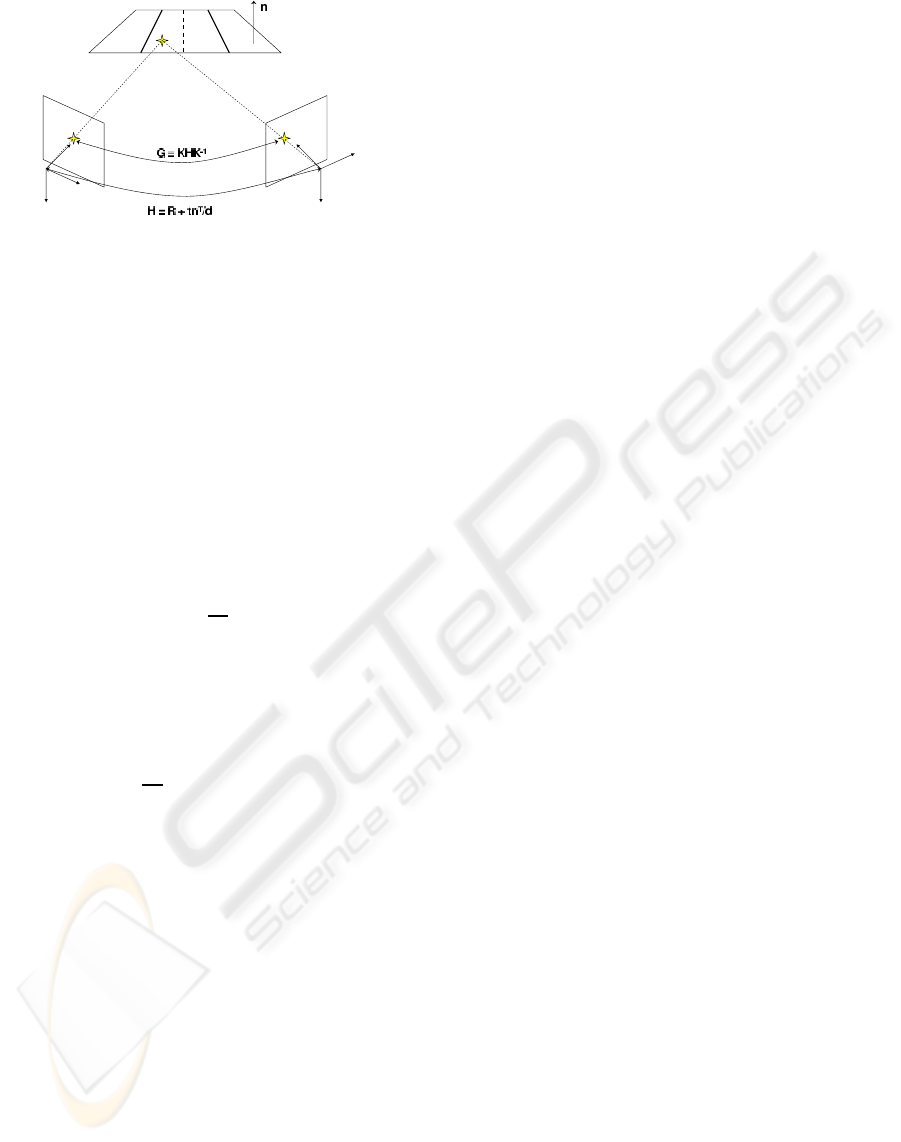
Figure 1: Perspective projection induced by a plane.
Let us now consider a second camera frame denoted
reference camera frame F
∗
in which the coordinates
of the same point P , in a similar manner as before,
are
∗
X =
∗
R
0
0
X+
∗
t
0
. (9)
By using Eq. (8) and Eq. (9), it is possible to relate the
coordinates of the same point P between reference F
∗
and current F
c
camera frames as
c
X =
c
R
0
∗
R
⊤
0
∗
X+
c
t
0
−
c
R
0
∗
R
⊤
0
∗
t
0
= (10)
=
c
R
∗
∗
X+
c
t
∗
However, considering that P lies on a plane Π, the
plane equation applied to the coordinates of the same
point in the reference camera frame gives us
∗
n
⊤∗
X = d
∗
⇔
1
d
∗
∗
n
⊤∗
X = 1 (11)
where,
∗
n
⊤
= [n
1
,n
2
,n
3
]
⊤
∈ R
3
is the unit normal
vector of the plane Π with respect to F
∗
and d
∗
∈ R
+
the distance from the plane Π to the optical center of
same frame. Thus, substituting Eq. (11) into Eq. (10)
results on
c
X =
c
R
∗
+
1
d
∗
c
t
∗
∗
n
⊤
∗
X =
c
H
∗
∗
X (12)
where,
c
H
∗
∈ R
3×3
is the so-called Euclidean homog-
raphy matrix. Applying the perspective projection
from Eq. (5) along with the Eq. (6) into the planar
homography mapping defined in Eq. (12), the rela-
tion between pixels coordinates p and
∗
p illustrated
in Figure 1 is obtained as follows
c
p ∝ K
c
H
∗
K
−1∗
p ∝
c
G
∗
∗
p (13)
where, G ∈ R
3×3
is the projectivehomography matrix
and ” ∝ ” denotes proportionality.
3 VISION-BASED AUTONOMOUS
APPROACH AND LANDING
3.1 Visual Tracking
The visual tracking is achieved by directly estimat-
ing the projective transformation between the image
taken from the airborne camera and a given reference
image. The reference images are then the key to re-
late the motion of the aircraft F
b
, through its airborne
camera F
c
, with respect to the earth frame F
0
. For
the PBVS scheme, it is the known pose of the refer-
ence camera with respect to the earth frame that will
allows us to reconstruct the aircraft position with re-
spect to the same frame. What concerns the IBVS,
where the aim is to reach a certain configuration ex-
pressed in terms of the considered feature, the path
planning is then an implicity need of such scheme.
For example, if lines are considered as features, the
path planning is defined as a function of the parame-
ters which define those lines. In the present case, the
path planning shall be defined by images because it is
the dense information that is used in order to estimate
the projective homography
c
G
∗
.
3.2 Visual Servoing
3.2.1 Linear Controller
The standard LQR optimal control technique was
chosen for the controller design, based on the lin-
earized models of both longitudinal and lateral mo-
tions in Eq. (4). Since not all the states are expected
to be driven to zero but to a given reference, the con-
trol law is more conveniently expressed as an opti-
mal output error feedback. The objective of the fol-
lowing vision-based control approaches is then to ex-
press the respective control laws as a function of the
visual information, which is directly or indirectly re-
lated with the pose of the aircraft. As a consequence,
the pose state vector P = [n,e,d,φ,θ,ψ]
⊤
∈ R
6
, in
agreement to the type of vision-based control ap-
proach, is given differently from the velocity screw
V = [u,v,w, p,q,r]
⊤
∈ R
6
, which could be provided
from an existent Inertial Navigation System (INS) or
from some filtering method based on the estimated
pose. Thus, the following vision-based control laws
are more correctly expressed as
u = −k
P
(P− P
∗
) − k
V
(V− V
∗
) (14)
where, k
P
and k
V
are the controller gains relative to
the pose and velocity states, respectively.
3.2.2 Position-based Visual Servoing
In the position-based, or 3D, visual servoing (PBVS)
the control law is expressed in the Cartesian space
and, as a consequence, the visual information com-
puted into the form of planar homography is used to
reconstruct explicitly the pose (position and attitude).
The airborne camera will be then considered as only
VISION-BASED AUTONOMOUS APPROACH AND LANDING FOR AN AIRCRAFT USING A DIRECT VISUAL
TRACKING METHOD
97

another sensor that provides a measure of the aircraft
pose.
In the same way that, knowing the relative pose
between the two cameras, R and t, and the planar
scene parameters, n and d, it is possible to compute
the planar homography matrix H it is also possible to
recover the pose from the decomposition of the esti-
mated projective homography G, with the additional
knowledge of the calibration matrix K. The decom-
position of H can be performed by singular value de-
composition (Faugeras, 1993) or, more recently, by an
analytical method (Vargas and Malis, 2007). These
methods result into four different solutions but only
two are physically admissible. The knowledge of the
normal vector n, which defines the planar scene Π,
allows us then to choose the correct solution.
Therefore, from the decomposition of the esti-
mated Euclidean homography
c
e
H
∗
= K
−1c
e
G
∗
K, (15)
both
c
e
R
∗
and
c
e
t
∗
/d
∗
are recovered being respectively,
the rotation matrix and normalized translation vector.
With the knowledge of the distance d
∗
, it is then pos-
sible to compute the estimated rigid-body relation of
the aircraft frame F
b
with respect to the inertial one
F
0
as
0
e
T
b
=
0
T
∗
b
T
c
c
e
T
∗
−1
=
0
e
R
b
0
e
t
b
0 1
(16)
where,
b
T
c
corresponds to the pose of the airborne
camera frame F
c
with respect to the aircraft body
frame F
b
and
0
T
∗
to the pose of the reference camera
frame F
∗
with respect to the earth frame F
0
. Finally,
without further considerations, the estimated pose
e
P
obtained from
0
e
R
b
and
0
e
t
b
could then be applied to
the control law in Eq. (17) as
u = −k
P
(
e
P− P
∗
) − k
V
(V− V
∗
) (17)
3.2.3 Image-based Visual Servoing
In the image-based, or 2D, visual servoing (IBVS)
the control law is expressed directly in the image
space. Then, in contrast with the previous approach,
the IBVS does not need the explicit aircraft pose rel-
ative to the earth frame. Instead, the estimated planar
homography
e
H is used directly into the control law
as some kind of pose information such that reach-
ing a certain reference configuration H
∗
the aircraft
presents the intended pose. This is the reason why an
IBVS scheme needs implicitly for path planning ex-
pressed in terms of the considered features.
In IBVS schemes, an important definition is that
of interaction matrix which is the responsible to relate
the time derivative of the visual signal vector s ∈ R
k
with the camera velocity screw
c
V
c∗
∈ R
6
as
˙
s = L
s
c
V
c∗
(18)
where, L
s
∈ R
k×6
is the interaction matrix, or the fea-
ture jacobian. Let us consider, for a moment, that
the visual signal vector s is a matrix and equal to the
Euclidean homography matrix
c
H
∗
, the visual feature
considered in the present paper. Thus, the time deriva-
tive of s, admitting the vector
∗
n/d
∗
as slowly vary-
ing, is
˙
s =
c
˙
H
∗
=
c
˙
R
∗
+
1
d
∗
c
˙
t
∗
∗
n
⊤
(19)
Now, it is known that both
c
˙
R
∗
and
c
˙
t
∗
are related with
the velocity screw
c
V
c∗
, which could be determined
using Eq. (3), as follows
c
b
V
c∗
=
c
˙
T
∗
c
T
−1
∗
= (20)
=
c
˙
R
∗
c
R
⊤
∗
c
˙
t
∗
−
c
˙
R
∗
c
R
⊤
∗
c
t
∗
0 1
from where,
c
˙
R
∗
=
c
b
ω
c
R
∗
and
c
˙
t
∗
=
c
v+
c
b
ω
c
t
∗
. By
using such results back in Eq. (19) results on
c
˙
H
∗
=
c
b
ω
c
R
∗
+
1
d
∗
c
t
∗
∗
n
⊤
+
1
d
∗
c
v
∗
n
⊤
=
=
c
b
ω
c
H
∗
+
1
d
∗
c
v
∗
n
⊤
(21)
Hereafter, in order to obtain the visual signal vector,
the stacked version of the homography matrix
c
˙
H
s
∗
must be considered and, as a result, the interaction
matrix is given by
˙
s =
c
˙
H
s
∗
=
I(3)
∗
n
1
/d
∗
−
c
b
H
∗1
I(3)
∗
n
2
/d
∗
−
c
b
H
∗2
I(3)
∗
n
3
/d
∗
−
c
b
H
∗3
c
v
c
ω
(22)
where, I(3) is the 3 × 3 identity matrix and H
i
is
the ith column of the matrix as well as n
i
is the
ith element of the vector. Note that,
b
ωH is the ex-
ternal product of ω with all the columns of H and
ω× H
1
= −H
1
× ω = −
b
H
1
ω.
However, the velocity screw in Eq. (18), as well
as in Eq. (22), denotes the velocity of the reference
frame F
∗
with respect to the airborne camera frame
F
c
and viewed from F
c
which is not in agreement
with the aircraft velocity screw that must be applied
into the control law in Eq. (17). Instead, the veloc-
ity screw shall be expressed with respect to the refer-
ence camera frame F
∗
and viewed from aircraft body
frame F
b
, where the control law is effectively applied.
In this manner, and knowing that the velocity tensor
c
b
V
c∗
is a skew-symmetric matrix, then
c
b
V
c∗
= −
c
b
V
⊤
c∗
= −
c
b
V
∗c
(23)
ICINCO 2009 - 6th International Conference on Informatics in Control, Automation and Robotics
98

Now, assuming the airborne camera frame F
c
rigidly
attached to the aircraft body frame F
b
, to change the
velocity screw from the aircraft body to the airborne
camera frame, the adjoint map must be applied as
c
b
V =
b
T
−1
c
b
b
V
b
T
c
= (24)
=
b
R
⊤
c
b
b
ω
b
R
c
b
R
⊤
c
b
v+
b
R
⊤
c
b
b
ω
b
t
c
0 0
from where,
b
R
⊤
c
b
b
ω
b
R
c
=
\
b
R
⊤
c
b
ω and
b
R
⊤
c
b
b
ω
b
t
c
=
−
b
R
⊤
c
b
b
t
c
c
ω and, as a result, the following velocity
transformation
c
W
b
∈ R
6×6
is obtained
c
V =
c
W
b
b
V =
b
R
⊤
c
−
b
R
⊤
c
b
b
t
c
0
b
R
⊤
c
b
v
b
ω
(25)
Using the Eq. (25) into the Eq. (22) along with the
result from Eq. (23) results as follows
˙
s =
c
˙
H
s
∗
= −L
s
c
W
b
b
V
∗c
(26)
Finally, let us consider the linearized version of the
previous result as
s− s
∗
=
c
H
s
∗
− H
∗s
= −L
s
c
W
b
b
W
0
(P− P
∗
) (27)
where,
b
W
0
=
S
0
0
0 R
0
(28)
are the kinematic and navigation equations, respec-
tively, linearized for the same trim point as for the air-
craft linear model [φ,θ,ψ]
⊤
0
= [0,θ
0
,0]
⊤
. It is then
possible to relate the pose error P− P
∗
of the air-
craft with the Euclidean homography error
c
H
s
∗
−H
∗s
.
For the present purpose, the reference configuration is
H
∗
= I(3) which corresponds to match exactly both
current I and reference I
∗
images. The proposed
homography-based IBVS visual control law is then
expressed as
u = −k
P
(L
s
c
W
0
)
†
c
e
H
s
∗
− H
∗s
− k
V
(V− V
∗
)
(29)
where, A
†
=
A
⊤
A
−1
A
⊤
is the Moore-Penrose
pseudo-inverse matrix.
4 RESULTS
The vision-based control schemes proposed above
have been developed and tested in an simulation
framework where the non-linear aircraft model is im-
plemented in Matlab/Simulink along with the control
aspects, the image processing algorithms in C/C++
and the simulated image is generated by the Flight-
Gear flight simulator. The aircraft model considered
Figure 2: Screenshot from the dense visual tracking soft-
ware. The delimited zone (left) corresponds to the bottom-
right image, warped to match with the top-right image. The
warp transformation corresponds to the estimated homogra-
phy matrix.
corresponds to a generic category B business jet air-
craft with 50m/s of stall speed, 265m/s of maximum
speed and 20m wing span. This simulation framework
has also the capability to generate atmospheric condi-
tion effects like fog and rain as well as vision sensors
effects like pixels spread function, noise, colorimetry,
distortion and vibration of different types and levels.
The chosen airport scenario was the Marseille-
Marignane Airport with an nominal initial position
defined by an altitude of 450m and a longitudinal
distance to the runway of 9500m, resulting into a
3 degrees descent for an airspeed of 60m/s. In order
to have illustrative results and to verify the robustness
of the proposed control schemes, two sets of simula-
tions results are presented. The first with an initial
lateral error of 50m, an altitude error of 30m and a
steady wind composed by 10m/s headwind and 1m/s
of crosswind. The latter, with a different initial lateral
error of 75m, considers in addition the presence of tur-
bulence. What concerns the visual tracking aspects, a
database of 200m equidistant images along the run-
way axis till the 100m height, and 50m after that,
was considered and the following atmospheric con-
ditions imposed: fog and rain densities of 0.4 and 0.8
([0,1]). The airborne camera is considered rigidly at-
tached to the aircraft and presents the following pose
b
P
c
= [4m, 0m, 0.1m,0,−8 degrees,0]
⊤
. The simula-
tion framework operates with a 50ms, or 20Hz, sam-
pling rate.
For all the following figures, the results of the two
simulations are presented simultaneously and iden-
tified in agreement with the legend in Figure 3(a).
When available, the corresponding references are pre-
sented in black dashed lines. Unless specified, the
detailed discussion of results is referred to the case
without turbulence.
Let us start with the longitudinal trajectory illustrated
in Figure 3(a) where it is possible to verify immedi-
ately that the PBVS results are almost coincident with
the ones where the sensor measurements were consid-
ered ideal (Sensors). Indeed, because the same con-
VISION-BASED AUTONOMOUS APPROACH AND LANDING FOR AN AIRCRAFT USING A DIRECT VISUAL
TRACKING METHOD
99
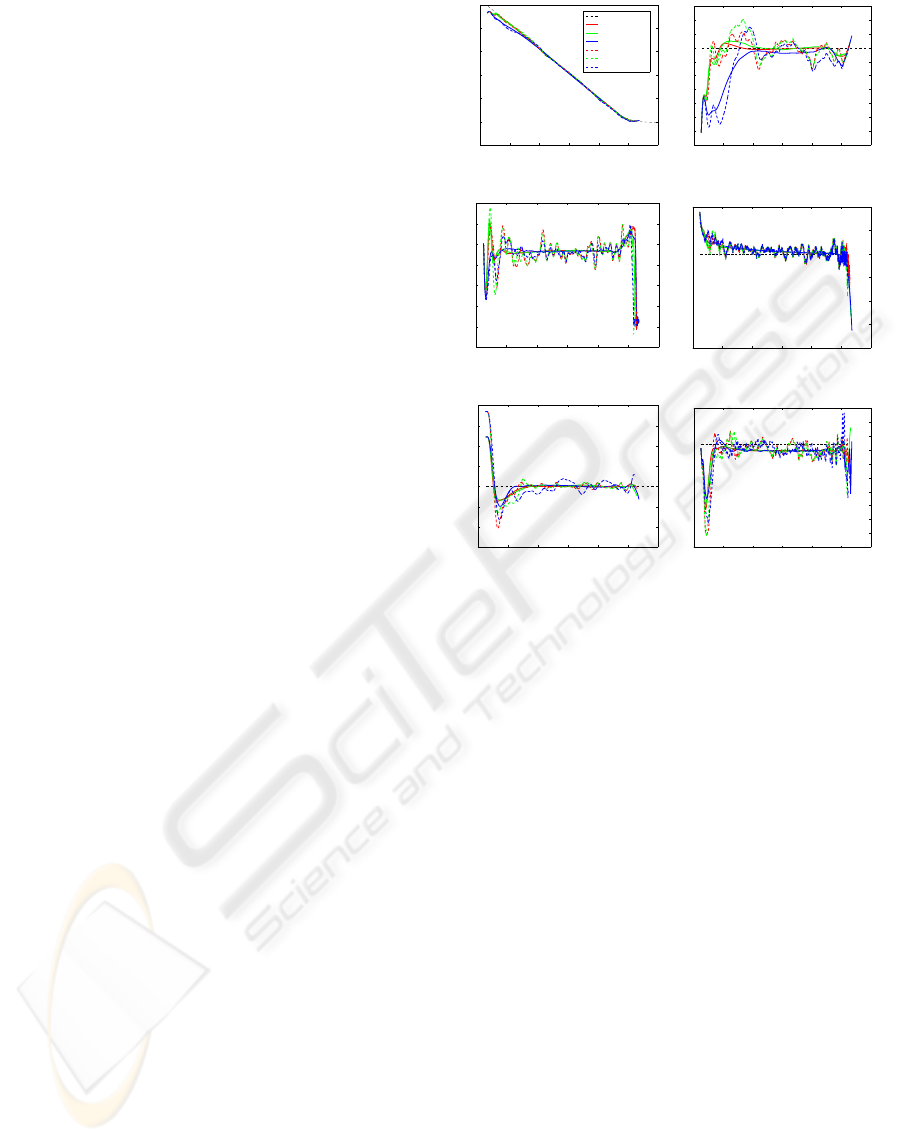
trol law is used for these two approaches, the results
differ only due to the pose estimation errors from the
visual tracking software. For the IBVS approach, the
first observation goes to the convergence of the air-
craft trajectory with respect to the reference descent
that occurs later than for the other approaches. This
fact is a consequence not only of the limited validity
of the interaction matrix in Eq (27), computed for a
stabilized descent flight, but also of the importance of
the camera orientation over the position, for high al-
titudes, when the objective is to match two images.
In more detail, the altitude error correction in Fig-
ure 3(b) shows then the IBVS with the slowest re-
sponse and, in addition, a static error not greater than
2m as a cause of the wind disturbance. In fact, the
path planning does not contemplates the presence of
the wind, from which the aircraft attitude is depen-
dent, leading to the presence of static errors. These
same aspects are verified in the presence of turbulence
but now with a global altitude error not greater than
8m, after stabilization. The increasing altitude error
at the distance of 650m before the touchdown corre-
sponds to the natural loss of altitude when proceeding
to the pitch-up, or flare, manoeuvre (see Figure 3(c))
in order to reduce the vertical speed and correctly land
the aircraft. What concerns the touchdown distances,
both Sensors and PBVS results are very close and at
a distance around 330m after the threshold line while,
for the IBVS, this distance is of approximately 100m.
In the presence of turbulence, these distances became
shorter mostly due to the oscillations in the altitude
control during the flare manoeuvre. Again, Sensors
and PBVS touchdown points are very close and about
180m from the runway threshold line while, for the
IBVS, this distance is about 70m.
The lateral trajectory illustrated in Figure 3(e) shows a
smooth lateral error correction for all the three control
schemes, where both visual control laws maintain an
error below the 2m after convergence. Once more, the
oscillations around the reference are a consequence of
pose estimation errors from visual tracking software,
which become more important near the Earth surface
due to the high displacement of the pixels in the im-
age and the violation of the planar assumption of the
region around the runway. The consequence of these
effects are perceptible in the final part not only in the
lateral error correction but also in the yaw angle of the
aircraft in Figure 3(f). For the latter, the static error is
also an influence of the wind disturbance which im-
poses an error of 1 degree with respect to the runway
orientation of exactly 134.8 degrees North.
In the presence of turbulence, Sensors and PBVS con-
trol schemes present a different behavior during the
−10000 −8000 −6000 −4000 −2000 0 2000
−100
0
100
200
300
400
500
Distance to Touchdown − [m]
Altitude − [m]
Reference
Sensors
PBVS
IBVS
Sensors w/ turb.
PBVS w/ turb.
IBVS w/ turb.
(a) Longitudinal trajectory
−10000 −8000 −6000 −4000 −2000 0 2000
−35
−30
−25
−20
−15
−10
−5
0
5
10
15
Distance to Touchdown − [m]
Altitude Error −[m]
(b) Altitude error
−10000 −8000 −6000 −4000 −2000 0 2000
−2
0
2
4
6
8
10
12
Distance to Touchdown − [m]
Pitch angle − [deg]
(c) Pitch angle
−10000 −8000 −6000 −4000 −2000 0 2000
40
45
50
55
60
65
70
Distance to Touchdown − [m]
True airspeed − [m/s]
(d) Airspeed
−10000 −8000 −6000 −4000 −2000 0 2000
−60
−40
−20
0
20
40
60
80
Distance to Touchdown − [m]
Lateral Error − [m]
(e) Lateral trajectory
−10000 −8000 −6000 −4000 −2000 0 2000
120
122
124
126
128
130
132
134
136
138
140
Distance to Touchdown − [m]
Yaw angle − [deg]
(f) Yaw angle
Figure 3: Results from the vision-based control schemes
(PBVS and IBVS) in comparison with the ideal situation of
precise measurements (Sensors).
lateral error correction manoeuvre. Indeed, due to the
important bank angle and the high pitch induced by
the simultaneous altitude error correction manoeuvre,
the visual tracking algorithm lost information on the
near-field of the camera essential for the precision of
the estimated translation. The resultant lateral error
estimative, greater than it really is, forces the lateral
controller to react earlier in order to minimize such
error. As for the longitudinal case, the IBVS presents
a slower response on position error corrections result-
ing into a lateral error not greater than 8m which con-
trasts with the 4m from the other two approaches.
It should be noted the precision of the dense visual
tracking software. Indeed, the attitude estimation er-
rors are often below 1 degree for transient responses
and below 0.1 degrees in steady state. Depending
on the quantity of information available in the near
field of the camera, the translation error could vary
between the 1m and 4m for both lateral and altitude
errors and between 10m and 70m for the longitudinal
distance. The latter is usually less precise due to its
alignment with the optical axis of the camera.
ICINCO 2009 - 6th International Conference on Informatics in Control, Automation and Robotics
100

5 CONCLUSIONS
In the present paper, two vison-based control schemes
for an autonomous approach and landing of an aircraft
using a direct visual tracking method are proposed.
For the PBVS solution, where the vision system is
nothing more than a sensor providing position and at-
titude measures, the results are naturally very similar
with the ideal case. The IBVS approach based on a
path planning defined by a sequence of images shown
clearly to be able to correct an initial pose error and
land the aircraft under windy conditions. Despite the
inherent sensitivity of the vision tracking algorithm to
the non-planarity of the scene and the high pixels dis-
placement in the image for low altitudes, a shorter dis-
tance between the images of reference was enough to
deal with potential problems. The inexistence of a fil-
tering method, as the Kalman filter, is the proof of the
robustness of the proposed control schemes and the
reliability of the dense visual tracking. This clearly
justify further studies to complete the validation and
the eventual implementation of this system on a real
aircraft.
ACKNOWLEDGEMENTS
This work is funded by the FP6 3rd Call European
Commission Research Program under grant Project
N.30839 - PEGASE.
REFERENCES
Azinheira, J., Rives, P., Carvalho, J., Silveira, G., de Paiva,
E.C., and Bueno, S. (2002). Visual servo control for
the hovering of an outdoor robotic airship. In IEEE In-
ternational Conference on Robotics and Automation,
volume 3, pages 2787–2792.
Behimane, S. and Malis, E. (2004). Real-time image-based
tracking of planes using efficient second-order mini-
mization. In IEEE International Conference on Intel-
ligent Robot and Systems, volume 1, pages 943–948.
Bourquardez, O. and Chaumette, F. (2007a). Visual servo-
ing of an airplane for alignment with respect to a run-
way. In IEEE International Conference on Robotics
and Automation, pages 1330–1355.
Bourquardez, O. and Chaumette, F. (2007b). Visual servo-
ing of an airplane for auto-landing. In IEEE Interna-
tional Conference on Intelligent Robots and Systems,
pages 1314–1319.
Chatterji, G., Menon, P., K., and Sridhar, B. (1998). Vision-
based position and attitude determination for aircraft
night landing. AIAA Journal of Guidance, Control and
Dynamics, 21(1).
Dickmanns, E. and Schell, F. (1992). Autonomous land-
ing of airplanes by dynamic machine vision. IEEE
Workshop on Application on Computer Vision, pages
172–179.
Faugeras, O. (1993). Three-dimensional computer vision: a
geometric view point. MIT Press.
Hamel, T. and Mahony, R. (2002). Visual servoing of
an under-actuated dynamics rigid-body system: an
image-based approach. In IEEE Transactions on
Robotics and Automation, volume 18, pages 187–198.
Kimmett, J., Valasek, J., and Junkins, J. L. (2002). Vi-
sion based controller for autonomous aerial refueling.
In Conference on Control Applications, pages 1138–
1143.
Mahony, R. and Hamel, T. (2005). Image-based visual
servo control of aerial robotic systems using linear im-
ages features. In IEEE Transaction on Robotics, vol-
ume 21, pages 227–239.
Malis, E. (2004). Improving vision-based control using ef-
ficient second-order minimization technique. In IEEE
International Conference on Robotics and Automa-
tion, pages 1843–1848.
Malis, E. (2007). An eficient unified approach to direct
visual tracking of rigid and deformable surfaces. In
IEEE International Conference on Robotics and Au-
tomation, pages 2729–2734.
Mati, R., Pollini, L., Lunghi, A., and Innocenti, M. (2006).
Vision-based autonomous probe and drogue aerial re-
fueling. In Conference on Control and Automation,
pages 1–6.
Proctor, A. and Johnson, E. (2004). Vision-only aircraft
flight control methods and test results. In AIAA Guid-
ance, Navigation, and Control Conference and Ex-
hibit.
Rives, P. and Azinheira, J. (2002). Visual auto-landing of
an autonomous aircraft. Reearch Report 4606, INRIA
Sophia-Antilopis.
Rives, P. and Azinheira, J. (2004). Linear structure follow-
ing by an airship using vanishing point and horizon
line in visual servoing schemes. In IEEE International
Conference on Robotics and Automation, volume 1,
pages 255–260.
Sharp, C., Shakernia, O., and Sastry, S. (2002). A vision
system for landing an unmanned aerial vehicle. In
IEEE International Conference on Robotics and Au-
tomation, volume 2, pages 1720– 1727.
Silveira, G., Azinheira, J., Rives, P., and Bueno, S. (2003).
Line following visual servoing for aerial robots com-
bined with complementary sensors. In IEEE Interna-
tional Conference on Robotics and Automation, pages
1160–1165.
Silveira, G. and Malis, E. (2007). Real-time visual tracking
under arbitrary illumination changes. In IEEE Con-
ference on Computer Vision and Pattern Recognition,
pages 1–6.
Vargas, M. and Malis, E. (2007). Deeper understanding of
the homography decomposition for vision-base con-
trol. Research Report 6303, INRIA Sophia-Antipolis.
VISION-BASED AUTONOMOUS APPROACH AND LANDING FOR AN AIRCRAFT USING A DIRECT VISUAL
TRACKING METHOD
101
