AN APPROACH OF ROBUST QUADRATIC STABILIZATION OF
NONLINEAR POLYNOMIAL SYSTEMS
Application to Turbine Governor Control
M. M. Belhaouane, R. Mtar, H. Belkhiria Ayadi and N. Benhadj Braiek
Laboratoire d’Etude et Commande Automatique de Processus - LECAP
´
Ecole Polytechnique de Tunis (EPT), BP.743, 2078 La Marsa, Tunis, Tunisie
Keywords:
Nonlinear polynomial systems, Lyapunov stability theory, Robust control, Power systems, Linear matrix in-
equalities.
Abstract:
In this paper, robust quadratic stabilization of nonlinear polynomial systems within the frame work of Linear
Matrix Inequalities (LMIs) is investigated. The studied systems are composed of a vectoriel polynomial func-
tion of state variable, perturbed by an additive nonlinearity which depends discontinuously on both time and
state. Our main objective is to show, by employing the Lyapunov stability direct method and the Kronecker
product properties, how a polynomial state feedback control law can be formulated to stabilize a nonlinear
polynomial systems and, at the same time, maximize the bounds on the perturbation which the system can
tolerate without going unstable. The efficiency of the proposed control strategy is illustrated on the Turbine -
Governor system.
1 INTRODUCTION
The problem of robust quadratic stabilization for non-
linear uncertain systems has attracted a consider-
able attention and several methods have been pro-
posed in the literature (Siljak, 1989) (Leitmann, 1993)
(Kokotovic and Arcak, 1999). In some very interest-
ing works, Lyapunov stability theory has been used
to design control laws for systems with structured or
unstructured parametric uncertainties and state pertur-
bations.
The basic principle of quadratic stabilization is to
find a feedback controller such that the closed-loop
system is stable with a fixed Lyapunov function. This
problem was initially proposed in (Barmish, 1985) to
study the control of uncertain systems satisfying the
so-called matching conditions. Since then, various re-
sults have been reported, including a necessary and
sufficient condition given in (Barmish, 1985) and the
Riccati equation method established in (Petersen and
Hollot, 1986). Particularly, they consider the class of
linear continuous systems subject to additive pertur-
bations which are nonlinear and discontinuous func-
tions in time and state of the system. The perturba-
tions are uncertain and all we know about them is that
they are contained within quadratic bounds.
Recently, the Linear Matrix Inequality (LMI) method
has been widely used in quadratic stabilization since
it can be solved efficiently using the interior-point
method (Boyd et al., 1994). In this fact, the quadratic
feedback stabilization of this type of systems using
LMI approach has received a great deal of atten-
tion in the Siljak-Stipanovic’works (Siljak and Sti-
panovic, 2000) (Stipanovic and Siljak, 2001) (Siljak
and Zecevic, 2005), in which sufficient conditions for
quadratic stabilizability are developed. Latter, a new
method which gives a less conservative result com-
pared to that of (Siljak and Stipanovic, 2000), by us-
ing a descriptor model transformation of the consid-
ered system, where an improved sufficient condition
for robust quadratic stabilization is given in terms
of Linear Matrix Inequality (LMI) (Zuo and Wang,
2005). However, the proposed results remain restric-
tives to the systems represented by a linear nominal
part and these conditions are rather difficult to check
and, in general, a nonlinear control law is required.
The main contribution of the present paper con-
sists in the replacement of the linear constant part by
a nonlinear polynomial function based on the Kro-
necker power of the state vector (Rotella and Tanguy,
1988) (Benhadj Braiek et al., 1995) (Brewer, 1978),
which has the advantage to approach any analytical
148
M. Belhaouane M., Mtar R., Belkhiria Ayadi H. and Benhadj Braiek N. (2009).
AN APPROACH OF ROBUST QUADRATIC STABILIZATION OF NONLINEAR POLYNOMIAL SYSTEMS - Application to Turbine Governor Control.
In Proceedings of the 6th International Conference on Informatics in Control, Automation and Robotics - Signal Processing, Systems Modeling and
Control, pages 148-155
DOI: 10.5220/0002213901480155
Copyright
c
 SciTePress

nonlinear systems and general enough to model many
physical systems (Benhadj Braiek and Rotella, 1992)
(Benhadj Braiek and Rotella, 1994) (Benhadj Braiek
et al., 1995) (Benhadj Braiek and Rotella, 1995)
(Benhadj Braiek, 1995) (Bouzaouache and Benhadj
Braiek, 2006). In another hand, we propose the use
of the LMI approach in terms of minimization prob-
lems (Belkhiria Ayadi and Benhadj Braiek, 2005) , to
derive a new sufficient LMI stabilization conditions,
which resolution yields a stabilizing polynomial con-
trol law involving the quadratic stabilization of the
polynomial closed-loop systems and the maximiza-
tion of the nonlinearity bounds. Notice that, in recent
years, various methods have been developed in field
of system analysis and control amount to compute
the controllers which enlarge the domain of attraction
of equilibrium points of polynomial systems through
LMI approach (Chesi et al., 1999). Mainly based on
LMI relaxation for solving polynomial optimizations
(Chesi et al., 2003) (Chesi, 2004), these methods
proposes a convex optimization solutions with LMI
constraints for a chosen Lyapunov functions (Chesi,
2009).
An additional contribution of this paper is to ap-
ply the versatile tools of LMI for the design of robust
feedback Turbine-Governor control (Anderson and
Fouad, 1977) (Elloumi, 2005). Our primary reason for
selecting this type of control is the underlying sys-
tem model, which can be bounded in a way that con-
forms to quadratic bounds of nonlinearity. The pro-
posed method has an advantage such as the control
design of our power system is formulated as a con-
vex optimization problem, which ensures computa-
tional simplicity, and guarantees the existence of a
solution. The optimal gains matrices are obtained di-
rectly, with no need for tuning parameters or trial and
error procedures.
This paper is organized as follows: section 2 is
devoted to introduce the description of the nonlin-
ear studied systems and problem formulation. In the
third section, the LMI sufficient condition for robust
quadratic stabilization of polynomial systems is pro-
posed. Applications to power systems are then con-
sidered in section 4. Finally some concluding remarks
are given in the last section.
2 DESCRIPTION OF THE
STUDIED SYSTEMS AND
PROBLEM FORMULATION
In the present paper, we focus on analytical non-
linear polynomial control-affine systems under non-
linear perturbations described by the following state
space equation:
˙
X = f (X(t)) +GU(t) + h(X (t),t)
=
r
∑
i=1
F
i
X
[i]
+ GU(t) + h(X(t),t),
(1)
where:
∀t ∈ R
+
; X ∈ R
n
is the state vector, U(t) ∈ R
m
is the
input vector.
For i = 1,...,r, X
[i]
∈ R
n
i
is the i-th Kronecker power
of the vector X and F
i
∈ R
n×n
i
are constant matrices.
G is a constant (n ×m) matrix and the polynomial de-
gree r is considered odd: r = 2s − 1, with s ∈ N
∗
.
h : R
n+1
→ R
n
is the nonlinear perturbations. The cru-
cial assumption about nonlinear function h(t, X(t)) is
that it is uncertain and all we know is that, in the do-
mains of continuity, it satisfies the quadratic inequal-
ity:
h
T
(t, X)h(t, X) ≤ α
2
X
T
H
T
HX, (2)
where α > 0 is the bounding parameter and H is a
constant matrix. For simplicity, we use h(t,X) instead
of h(t, X(t)) .
A large amount of works have been developed in
the robust quadratic stabilization area, considering
a particular class of nonlinear systems, where the
nonlinearities are totally in the perturbation terms
(Stipanovic and Siljak, 2001) (Siljak and Zece-
vic, 2005) (Zuo and Wang, 2005). The basic idea
addressed in this paper is the consideration of a non-
linear uncertain systems described by a polynomial
part with nonlinear perturbations which present the
uncertainties (Mtar et al., 2007). The present work is
an attempt towards expanding the robust quadratic
stabilization approach of the considered nonlinear
systems in the literature to polynomial ones. The aim
of the proposed approach is to guarantees on the
one hand, the stabilization of the linear part of the
polynomial system, and on the other hand to weaken
the perturbation which provide the maximization of
the domain of uncertainties.
3 ROBUST STABILIZING
CONTROL SYNTHESIS USING
THE LMI APPROACH
When the linear part of the perturbed polynomial sys-
tem (1) (defined by F
1
) is not stable, we can introduce
a nonlinear feedback to stabilize the overall system
and, at the same time, maximize its tolerance to uncer-
tain nonlinear perturbations. The considered polyno-
AN APPROACH OF ROBUST QUADRATIC STABILIZATION OF NONLINEAR POLYNOMIAL SYSTEMS -
Application to Turbine Governor Control
149

mial control law is described by the following equa-
tion:
U = k(X) =
r
∑
i=1
K
i
X
[i]
, (3)
where K
i,i=1,...,r
are constant gains matrices, which
stabilizes asymptotically and globally the equilibrium
(X = 0) of the considered system.
When we apply the feedback (3) to the open-loop sys-
tem (1), we obtain the closed-loop system:
˙
X = ( f + Gk)(X ) + h(t, X)
= a(X) + h(t, X)
=
r
∑
i=1
A
i
X
[i]
+ h(t,X)
(4)
where:
A
i
= F
i
+ GK
i
(5)
is the closed-loop system matrix.
We define the following set:
S(h, H,α) = {h : h
T
(t, X)h(t, X) ≤ α
2
X
T
H
T
HX}.
(6)
For any given matrix H, our purpose is to establish
robust quadratic stabilization of the system (4-5) and
meanwhile make the set S(h,H,α) as large as possi-
ble.
Definition 1. The system (1) is robustly stabilized by
the control law (3) if the closed-loop system (4) is ro-
bustly stable with degree α for all h(t, X) satisfying
constraint (2).
Using the quadratic Lyapunov function:
V (X) = X
T
PX,
(7)
which is positive definite when P is a symmetric
positive definite (n × n) matrix and computing the
derivative
˙
V (X) along the trajectory of the system (4),
lead to the sufficient condition of the global asymp-
totic stabilization of the perturbed polynomial sys-
tem. Useful mathematical transformations have al-
lowed the formulation of the obtained condition as an
LMI optimization problem according to the polyno-
mial system parameters, given by the following The-
orem 1:
Theorem 1. The system (4) is robustly stabilized by
control law (3) if the following optimization problem
is feasible:
minimize η =
1
α
2
subject to D
S
(P) > 0, γ > 0






Π(P) ? ? ? ?
ΛD
S
(P)τ −I 0 0 0
D
S
(P)τ 0 −
1
γ
I 0 0
G
˜
M (k)τ 0 0 −
1
γ
I 0
HΛτ 0 0 0 −ηI






< 0 (8)
where: η =
1
α
2
and
˜
M (k) = γ
−1
M (k).
? : denotes the elements below the main diagonal of
a symmetric block matrix.
The relative notations of the Theorem 1 are men-
tioned in Appendix A.3.
To prove the Theorem 1, we need the two following
lemmas:
Lemma 1. (Yakubovich, 1977)
Let Ω
0
(x) and Ω
1
(x) be two arbitrary quadratic forms
over R
n
, then Ω
0
(x) < 0 for all x ∈ R
n
−{0} satisfying
Ω
1
(x) ≤ 0 if and only if there exist σ ≥ 0 such that:
Ω
0
(x) − σΩ
1
(x) < 0, ∀x ∈ R
n
− {0} (9)
Lemma 2. (Zhou and Khargonedkar, 1988)
For any matrices A and B with appropriate dimen-
sions and for any positive scalar γ > 0, one has:
A
T
B + B
T
A ≤ γA
T
A + γ
−1
B
T
B (10)
Proof of Theorem 1:
Let us consider the quadratic Lyapunov function (7)
and differentiating along trajectory of the system (4),
we have:
˙
V (X) =
˙
X
T
PX +X
T
P
˙
X
= X
T
P(
r
∑
i=1
A
i
X
[i]
+ h(t,X))
+ (
r
∑
i=1
A
i
X
[i]
+ h(t,X))
T
PX
=
r
∑
i=1
(X
T
PA
i
X
[i]
+ X
[i]T
A
T
i
PX)
+ h
T
PX +X
T
Ph
= 2
r
∑
i=1
X
T
PA
i
X
[i]
+ h
T
PX +X
T
Ph.
(11)
Using the rule of the vec-function (see Appendix A.1),
one obtains:
˙
V (X) = 2
r
∑
i=1
Ψ
T
i
X
[i+1]
+ h
T
PX +X
T
Ph,
(12)
where:
Ψ
i
= vec(PA
i
).
(13)
Then, we have:
˙
V (X) = 2X
T
D
S
(P)M (a)X + h
T
PX +X
T
Ph
= X
T
[D
S
(P)M (a) + M (a)
T
D
S
(P)]X
+ h
T
PX +X
T
Ph,
(14)
ICINCO 2009 - 6th International Conference on Informatics in Control, Automation and Robotics
150

where D
S
(P) and M (a) are defined in Appendix, and
X is expressed by the following equation:
X =
h
X
T
X
[2]
T
·· · X
[s]
T
i
T
(15)
For more details, the transitions between the inequali-
ties (12) to (14) are detailed in (Benhadj Braiek, 1996)
(Belhaouane et al., 2008).
When considering the nun-redundant form, the vector
X can be written as:
X = τ
˜
X , (16)
where τ is mentioned in Appendix A.3.
Consequently,
˙
V (X) can be expressed as:
˙
V (X ) =
e
X
T
τ
T
(D
S
(P)M (a) + M (a)
T
D
S
(P))τ
e
X
+ h
T
PX +X
T
Ph
(17)
Which can be written as:
˙
V (X ) =
e
X
T
τ
T
(D
S
(P)M (a) + M (a)
T
D
S
(P))τ
e
X
+ h
T
ΛD
S
(P)τ
e
X +
e
X
T
τ
T
D
S
(P)Λh,
(18)
with Λ is mentioned in Appendix A.3.
A sufficient condition of the global quadratic stabi-
lization of the equilibrium (X = 0) is that (18) is neg-
ative definite. Considering the obtained result, we can
derive LMI sufficient conditions for global asymp-
totic stabilization of the studied system by employing
some LMI techniques given by the following devel-
opment:
Using the S-procedure method, presented by the
Lemma1, the inequality (18) with the constraint
h
T
h − α
2
e
X
T
(HΛτ)
T
(HΛτ)
e
X ≤ 0 derived from (2), is
equivalent to the existence of a D
S
(P) matrix and a
scalar ε ≥ 0 such that:
e
X
T
τ
T
(D
S
(P)M (a) + M (a)
T
D
S
(P))τ
e
X + h
T
ΛD
S
(P)τ
e
X
+
e
X
T
τ
T
D
S
(P)Λh − ε[h
T
h − α
2
e
X
T
(HΛτ)
T
(HΛτ)
e
X ] < 0
which can be written as:

e
X
T
h
T

T

Q
11
+ εα
2
(HΛτ)
T
(HΛτ) ?
ΛD
S
(P)τ −εI

e
X
h

< 0
(19)
where:
Q
11
= τ
T
(D
S
(P)M (a) + M (a)
T
D
S
(P))τ. It should be
noted that inequality (19) is a non-strict LMI since
ε ≥ 0. For the minimization problem, it is well-known
in (Boyd et al., 1994), that the minimization result
under non-strict LMI constraints is equivalent to that
under strict LMI constraints. Thus we can substitute
ε > 0 by ε ≥ 0. Then, the inequality (19) is further
equivalent to the existence of a matrix
ˆ
D
S
(P) so that:
ˆ
D
S
(P) > 0

ˆ
Q
11
+ α
2
(HΛτ)
T
(HΛτ) ?
Λ
ˆ
D
S
(P)τ −I

< 0 (20)
where
ˆ
P = ε
−1
P and
ˆ
D
S
(P) = ε
−1
D
S
(P).
In what follows, the matrix
ˆ
D
S
(P) is replaced by
D
S
(P), to relieve the writing.
According to the following relation (see the lemma
given in (Benhadj Braiek et al., 1995)):
M (a) = M ( f + Gk) = M ( f ) + GM (k), (21)
we can write:

S
11
+ R
11
?
ΛD
S
(P)τ −I

< 0 (22)
where:
S
11
= Π(P) + α
2
(HΛτ)
T
(HΛτ),
R
11
= τ
T
(D
S
(P)GM (k) + (D
S
(P)GM (k))
T
)τ
and Π(P) = τ
T
(D
S
(P)M ( f ) + M ( f )
T
D
S
(P))τ.
G, D
S
(P), M ( f ) and M (k) are mentioned in Ap-
pendix A.3.
Using the well known matrix inequality given by
Lemma 2, it follows that (22) holds if there exist a
constant symmetric matrix D
S
(P) > 0 and a positive
scalar γ > 0, such that:

S
11
+ R
0
11
?
ΛD
S
(P)τ −I

< 0 (23)
where:
R
0
11
= γ τ
T
D
S
(P)
T
D
S
(P)τ + γ
−1
τ
T
M (k)
T
G
T
GM (k)τ
1
.
Relying on the generalized Schur Complement, equa-
tion (23) can be rewritten as:




Π(P) + α
2
(HΛτ)
T
(HΛτ) ? ? ?
ΛD
S
(P)τ −I 0 0
D
S
(P)τ 0 −
1
γ
I 0
GM (k)τ 0 0 −γI




< 0
(24)
Pre-multiplying and post-multiplying:
Φ = diag(I,I,I, γ
−1
I)
for both sides of (24), we have:




Π(P) + α
2
(HΛτ)
T
(HΛτ) ? ? ?
ΛD
S
(P)τ −I 0 0
D
S
(P)τ 0 −
1
γ
I 0
G
˜
M (k)τ 0 0 −
1
γ
I




< 0
(25)
where
˜
M (k) = γ
−1
M (k) and
˜
K
i
= γ
−1
K
i
.
Finally, by using the Schur complement, we get:






Π(P) ? ? ? ?
ΛD
S
(P)τ −I 0 0 0
D
S
(P)τ 0 −
1
γ
I 0 0
G
˜
M (k)τ 0 0 −
1
γ
I 0
HΛτ 0 0 0 −ηI






< 0 (26)
where η =
1
α
2
.
To establish robust quadratic stabilization in the sense
AN APPROACH OF ROBUST QUADRATIC STABILIZATION OF NONLINEAR POLYNOMIAL SYSTEMS -
Application to Turbine Governor Control
151

of Definition 1 of the system (4) under the constraint
(2) with maximal α, it comes the following optimiza-
tion problem:



minimize η =
1
α
2
s.t. (26)
γ > 0,D
S
(P) > 0,P > 0
(27)
translated by the Theorem1, which ends the proof.
4 APPLICATION TO POWER
SYSTEM CONTROL
To illustrate how the proposed LMI approach can
be applied for the robust feedback control of power
systems, we will consider a electrical mono-machine
system with steam valve control (see Figure 1). The
parameters of the considered system are given by the
following list of symbols:
δ : rotor angle for machine, in radian;
ω : relative speed for machine, in radian/s;
P
m
: mechanical power for machine, in pu;
P
c
: power control input of machine, in pu;
X
e
: steam valve opening for machine, in pu;
H : inertia constant for machine, in second;
D : damping coefficient for machine, in pu;
T
m
: time constant of machine’s turbine of machine,
in second;
T
e
: time constant of machine’s speed governor, in
second;
K
m
: gain of machine turbine;
R : regulation constant of machine, in pu;
E : internal transient voltage for machine, in pu;
B : nodal susceptance for machine, in pu;
ω
0
: the synchronous machine speed, in radian/s;
δ
0
, P
m
0
and X
e
0
are the initial values of δ(t), P
m
(t)
and X
e
(t) respectively.
The generator dynamics are described as (Sauer
and Pai, 1998) (Siljak and Zecevic, 2002):
˙
δ = ω
˙
ω = −
D
2H
ω +
ω
0
2H
(P
m
− EV Bsinδ).
(28)
The equation linking the mechanical power P
m
to the
steam valve opening of turbine X
e
for synchronous
machine is:
˙
P
m
= −
1
T
m
P
m
+
K
m
T
m
X
e
. (29)
The mechanical-hydraulic speed governor can be rep-
resented as first order system:
˙
X
e
= −
K
e
T
e
Rω
0
ω −
1
T
e
X
e
+
1
T
e
P
c
, (30)
+
-
Local speed
regulator
P
c
ω
Valve Turbine
Gain
Generator
ω
+
-
P
m
P
m
0
δ
∆
P
m
+
-
0
∆δδ
+
-
X
0
∆
e
X
e
X
e
Figure 1: Diagram Bloc representation of Electrical Mono-
machine System.
where the term P
c
represents the control input.
Defining new states:

∆δ(t) ω(t) ∆P
m
(t) ∆X
e
(t)

T
(31)
as deviations from the equilibrium,
where:
∆δ(t) = δ(t) − δ
0
; ∆P
m
(t) = P
m
(t) − P
m
0
∆X
e
(t) = X
e
(t) − X
e
0
.
Then, we obtain the modified system given by the fol-
lowing state space equation:
˙
X(t) = AX(t) + B
0
U +h(t, X), (32)
where:
A =




0 1 0 0
0
−D
2H
ω
0
2H
0
0 0 −
1
T
m
K
m
T
m
0 −
K
e
T
e
Rω
0
0 −
1
T
e




B
0
= (0 0 0
1
T
e
)
T
and
h(t, X) =



0
−ω
0
EV B/2H
0
0



g(X(t)),
with g(X(t)) = sinδ(t) −sinδ
0
, represents the nonlin-
earity of system (32).
The nonlinear system (32) can be developed into a
polynomial form by a Taylor series expansions, then
we obtain the new state space representation given by
the following form:
˙
X = F
1
X +F
2
X
[2]
+ F
3
X
[3]
+ GU(t) + h(t,X),
(33)
where:
F
1
=




0 1 0 0
−ω
0
EV B/2H
−D
2H
ω
0
2H
0
0 0 −
1
T
m
K
m
T
m
0 −
K
e
T
e
Rω
0
0 −
1
T
e




ICINCO 2009 - 6th International Conference on Informatics in Control, Automation and Robotics
152

F
2
= 0
4×16
, F
3
(2,1) =
ω
0
EV B
12H
.
For the others values:
F
3
(i, j) = 0 ∀i, j : (i = 1,...4; j = 1,...64)
G = B
0
and
h(t, X) =



0
−ω
0
EV B/2H
0
0



g(X(t)), (34)
where:
g(X(t)) = sinδ(t) − δ(t) +
δ(t)
3
6
. (35)
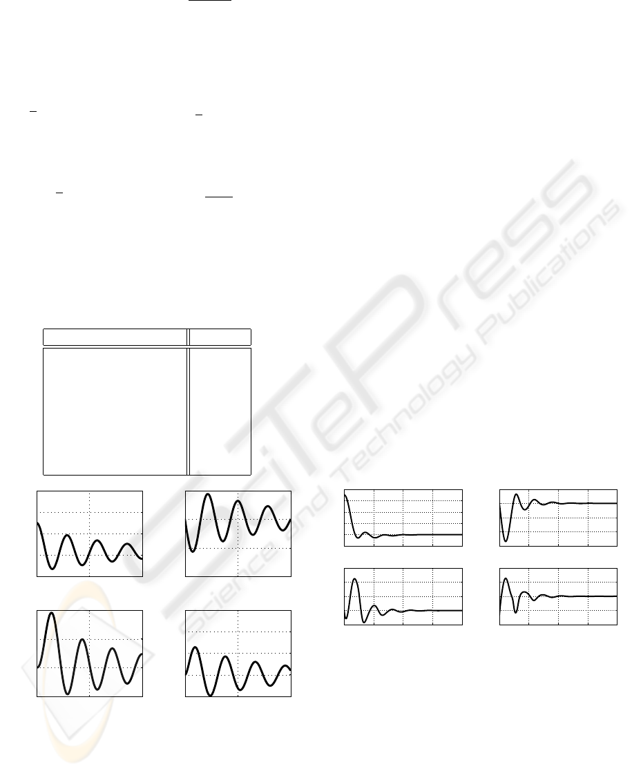
According the values of the machine parameters
(Sauer and Pai, 1998) indicated in Table 1, the evo-
lution of the state variables of system (33) is shown
in the Figure 2. Since the nonlinearity (34) of system
Table 1: Machine system parameters.
Symbols of parameters Values
H(s) 5.1
D(pu) 3
T
m
(s) 0.35
T
e
(s) 0.1
R 0.05
K
m
1
K
e
1
ω
0
(rad/s) 314.159
0 2 4
0.2
0.4
0.6
0.8
1
time(s)
∆ δ (rad)
0 2 4
−2
−1
0
1
temps(s)
w (rad/s)
0 2 4
−0.02
0
0.02
0.04
temps(s)
∆ Pm (pu)
0 2 4
−0.05
0
0.05
0.1
0.15
temps(s)
∆ Xe (pu)
Figure 2: Evolution of state variables towards an perturba-
tion on the variable δ.
(33) satisfy the quadratic inequality (2) with H = I,
the LMI robust stabilizing control given by Theorem
1 can be applied to considered power system in order
to maximize the domain of nonlinearity while ensur-
ing the stability of the overall system.
The solution of problem (27) yields to the uncertainty
bound α
max
= 0.4834 and
P =



10.0734 5.3037 −3.2516 1.8013
5.3037 6.0628 −4.6859 1.2175
−3.2516 −4.6859 9.7071 −2.1715
1.8013 1.2175 −2.1715 12.3111



The control law gain matrices, extracted from M (k),
are given by:
K
1
=

−86.592 −87.171 −90.911 −89.173

T
- For i = 1,..., 16 :
K
2
(1) = −216.909, K
2
(2) = K
2
(5) = −40.431
K
2
(3) = K
2
(4) = K
2
(7) = K
2
(8) = K
2
(9) = −49.443
K
2
(10) = K
2
(12) = K
2
(13) = K
2
(14) = K
2
(15) = −49.443
K
2
(11) = K
2
(16) = −96.292.
- For i = 1,..., 64 :
K
3
(1) = K
3
(17) = K
3
(33) = K
3
(49) = −216.909
K
3
(2) = K
3
(5) = K
3
(18) = K
3
(21) = −40.431
K
3
(34) = K
3
(37) = K
3
(50) = K
3
(53) = −40.431
K
3
(3) = K
3
(4) = K
3
(7) = K
3
(8) = −49.443
K
3
(9) = K
3
(10) = K
3
(12) = K
3
(13) = K
3
(14) = −49.443
K
3
(15) = K
3
(19) = K
3
(20) = K
3
(23) = K
3
(24) = −49.443
K
3
(25) = K
3
(26) = K
3
(28) = K
3
(29) = K
3
(30) = −49.443
K
3
(31) = K
3
(35) = K
3
(36) = K
3
(39) = K
3
(40) = −49.443
K
3
(41) = −49.443 = K
3
(42) = K
3
(44) = K
3
(45) = −49.443
K
3
(46) = K
3
(47) = K
3
(51) = K
3
(52) = K
3
(55) = −49.443
K
3
(56) = K
3
(57) = K
3
(58) = K
3
(60) = K
3
(61) = −49.443
K
3
(62) = K
3
(63) = −49.443
K
3
(6) = K
3
(11) = K
3
(16) = K
3
(22) = K
3
(27) = −96.292
K
3
(32) = K
3
(38) = K
3
(43) = K
3
(54) = K
3
(59) = −96.292
K
3
(64) = −96.292
0 1 2 3 4
−0.2
0
0.2
0.4
0.6
0.8
time(s)
∆ δ (rad)
0 1 2 3 4
−3
−2
−1
0
1
temps(s)
w (rad/s)
0 1 2 3 4
−0.2
0
0.2
0.4
0.6
temps(s)
∆ Pm (pu)
0 1 2 3 4
−2
−1
0
1
2
temps(s)
∆ Xe (pu)
Figure 3: Closed-loop responses of the power system with
polynomial control.
From the simulation results shown in Figure 3, it
is obvious that the results confirm the validity of the
proposed method and the uncertainty bound found by
the LMI procedure (27), dominates the maximum of
the perturbation function (35) of the system (33). The
polynomial robust control can rapidly damp the os-
cillations of the studied system and greatly enhance
transient stability of the mono-machine power sys-
tem. Besides, the polynomial control is more reassur-
ing in the case of a more aggressive perturbation.
AN APPROACH OF ROBUST QUADRATIC STABILIZATION OF NONLINEAR POLYNOMIAL SYSTEMS -
Application to Turbine Governor Control
153

5 CONCLUSIONS
A sufficient LMI condition for robust quadratic stabi-
lization of polynomial systems under nonlinear per-
turbations has been proposed in this work. This new
feedback stabilizing approach is based on the direct
Lyapunov method and elaborated algebraic develop-
ments using the Kronecker product properties. These
developments have been turned into an LMI min-
imization problem, which can be easily solved by
means of numerically efficient convex programming
algorithms. A mono-machine power system is consid-
ered as an application example of the technique devel-
oped in this paper. The numerical simulation results
have confirmed the efficiency of the proposed poly-
nomial controller which can rapidly damp the system
oscillations and greatly enhance the transient stability
of the considered mono-machine power system de-
spite the nonlinear uncertainty affecting the studied
system.
REFERENCES
Anderson, P. M. and Fouad, A. A. (1977). Power system
control and stability. The IOWA.
Barmish, B. (1985). Necessary and sufficient conditions for
quadratic stabilizability of an uncertain systems. Jour-
nal of Optimization Theory and Applications, 46:399–
408.
Belhaouane, M., Mtar, R., Belkhiria Ayadi, H., and Benhadj
Braiek, N. (2008). An LMI technique for the global
stabilization of nonlinear polynomial systems. Inter-
national Journal of Computers, Communication and
Control (IJCCC), to appear.
Belkhiria Ayadi, H. and Benhadj Braiek, N. (2005). On
the robust stability analysis of uncertain polynomial
systems: an LMI approach. 17th IMACS World
Congress, Scientific Computation, Applied Mathemat-
ics and Simulation.
Benhadj Braiek, N. (1995). Feedback stabilization and sta-
bility domain estimation of nonlinear systems. Jour-
nal of The Franklin Institute, 332(2):183–193.
Benhadj Braiek, N. (1996). On the global stability of non-
linear polynomial systems. IEEE Conference On De-
cision and Control,CDC’96.
Benhadj Braiek, N. and Rotella, F. (1992). Robot model
simplification by means of an identtification method.
Robotics and Flexible Manufacturing Systems, Edit. J.
C. Gentina and S. G. Tzafesta, pages 217–227.
Benhadj Braiek, N. and Rotella, F. (1994). State observer
design for analytical nonlinear systems. IEEE Syst.
Man and Cybernetics Conference, 3:2045–2050.
Benhadj Braiek, N. and Rotella, F. (1995). Stabilization
of nonlinear systems using a Kronecker product ap-
proach. European Control Conference ECC’95, pages
2304–2309.
Benhadj Braiek, N., Rotella, F., and Benrejeb, M. (1995).
Algebraic criteria for global stability analysis of non-
linear systems. Journal of Systems Analysis Modelling
and Simulation, Gordon and Breach Science Publish-
ers, 17:221–227.
Bouzaouache, H. and Benhadj Braiek, N. (2006). On
guaranteed global exponential stability of polynomial
singularly perturbed control systems. International
Journal of Computers, Communications and Control
(IJCCC), 1(4):21–34.
Boyd, S., Ghaoui, L., and Balakrishnan, F. (1994). Lin-
ear Matrix Inequalities in System and Control Theory.
SIAM.
Brewer, J. (1978). Kronecker product and matrix calculus
in system theory. IEEE Trans.Circ.Sys, CAS-25:722–
781.
Chesi, G. (2004). Estimating the domain of attrac-
tion for uncertain polynomial systems. Automatica,
40(11):1981–1986.
Chesi, G. (2009). Estimating the domain of attraction for
non-polynomial systems via LMI optimizations. Au-
tomatica, doi:10.1016/j.automatica.2009.02.011(in
press).
Chesi, G., Garulli, A., Tesi, A., and Vicino, A. (2003).
Solving quadratic distance problems: an lmi-based
approach. IEEE Transactions on Automatic Control,
48(2):200–212.
Chesi, G., Tesi, A., Vicino, A., and Genesio, R. (1999). On
convexification of some minimum distance problems.
5th European Control Conference ECC’99.
Elloumi, S. (2005). Commande d
´
ecentralis
´
ee robuste des
syst
`
emes non lin
´
eaires interconnect
´
es: Application
`
a un syst
`
eme de production-transport de l’
´
energie
´
el
´
ectrique multi-machines. Th
`
ese de doctorat es sci-
ences, Ecole Nationale d’Ing
´
enieurs de Tunis.
Kokotovic, P. and Arcak, M. (1999). Constructive nonlin-
ear control: Progress in the 90’s. Proceedings of the
14th IFAC World Congress, Beijing, P.R. China, Ple-
nary Volume:49–77.
Leitmann, G. (1993). On one approach to the control of un-
certain systems. Journal of Dynamic Systems, Mea-
surement and Control, 115:373–380.
Mtar, R., Belkhiria Ayadi, H., and Benhadj Braiek, N.
(2007). Robust stability analysis of polynomial sys-
tems under nonlinear perturbations: an LMI ap-
proach. Fourth Inernational Multi-conference on Sys-
tems, Signals and Devices (SSD’07).
Petersen, I. and Hollot, C. (1986). A Riccati equation ap-
proach to the stabilization of uncertain linear systems.
Automatica, 22:397–411.
Rotella, F. and Tanguy, G. (1988). Non linear sys-
tems: identification and optimal control. Int.J.Control,
48(2):525–544.
Sauer, P. W. and Pai, M. A. (1998). Power system dynamics
and stability. Englewood Cliffs, NJ:Prentice-Hall.
Siljak, D. (1989). Parameter space methods for robust con-
trol design: A guided tour. IEEE Transactions on Au-
tomatic Control, 34:674–688.
Siljak, D. and Stipanovic, D. (2000). Robust stabilization of
nonlinear systems: The LMI approach. Mathematical
Problems in Engineering, 6:461–493.
ICINCO 2009 - 6th International Conference on Informatics in Control, Automation and Robotics
154

Siljak, D. and Zecevic, A. (2005). Control of large-scale
systems: Beyond decentralized feedback. Annual Re-
views in Control, 29:169–179.
Siljak, D. and Zecevic, D. M. S. A. (2002). Robust decen-
tralized turbine/governor control using linear matrix
inequalities. IEEE Transactions On Power Systems,
17(3):715–722.
Stipanovic, D. and Siljak, D. (2001). Robust stability
and stabilization of discrete-time nonlinear systems:
The LMI approach. International Journal of Control,
74:873–879.
Yakubovich, V. (1977). S-procedure in nonlinear control
theory. Vestnick Leningrad Univ. Math.,, 4:73–93.
Zhou and Khargonedkar (1988). Robust stabilization of lin-
ear systems with norm-bounded time-varying uncer-
tainty. Sys. Contr. Letters, 10:17–20.
Zuo, Z. and Wang, Y. (2005). A descriptor system ap-
proach to robust quadratic stability and stabilization
of nonlinear systems. IEEE International Conference
on Systems, Man and Cybernetics, 1:486–491.
APPENDIX
The dimensions of the matrices used in this section
are the following: A(p × q), C(q × f ), E(n × p)
A.1- vec(.) function:
An important vector valued function of matrix de-
noted vec(.) was defined in (Brewer, 1978) as follows:
A =

A
1
A
2
... A
q

∈ R
p×q
,
where
∀i ∈
{
1,..., q
}
, A
i
∈ R
p
vec(A) = [A
1
A
2
.. . A
q
]
T
∈ R
pq
.
We recall the following useful rule (Brewer, 1978) of
vec-function:
vec(EAC) = (C
T
⊗ E)vec(A)
A.2- mat(.) function:
A special function mat
(n,m)
(.) can be defined as fol-
lows:
If V is a vector of dimension p = n.m then M =
mat
(n,m)
(V ) is the (n × m) matrix verifying V =
vec(M).
A.3- Notations related to Theorem 1:
(i).
τ =






T
1
T
2
0
T
3
0
.
.
.
T
s






where:
∀i ∈ N; ∃! T
i
∈ R
n
i
×n
i
, such as X
[i]
= T
i
˜
X
[i]
,
with:
˜
X
[i]
represents the nun-redundant i-power of X
(Benhadj Braiek et al., 1995).
(ii).
Λ =

I
n
0
n×n
2
·· · 0
n×n
s

,
verifying X =
˜
X =
˜
Λ
˜
X , Λ
T
P = D
s
(P)Λ
T
where:
˜
Λ = Λτ.
(iii).
D
s
(P) =




P 0
P ⊗ I
n
.
.
.
0 P ⊗ I
n
s−1




(iv).
G =




G 0
G ⊗ I
n
.
.
.
0 G ⊗ I
n
s−1




(v).
Π(P) = D
S
(P)M ( f ) + M ( f )
T
D
S
(P),
where for a polynomial vectorial function:
z(X ) =
r
∑
i=1
Z
i
X
[i]
,
with X ∈ R
n
and Z
i
are (n × n
i
) constant matrices.
We define the (υ × υ) matrix M (z) by:
M (z) =













M
11
(Z
1
) M
12
(Z
2
) 0 ... 0
0 M
22
(Z
3
)
.
.
.
.
.
.
.
.
.
.
.
.
.
.
.
.
.
.
.
.
.
0
.
.
.
.
.
.
M
s−1,s−1
(Z
2s−3
) M
s−1,s
(Z
2s−2
)
0 ... ... 0 M
s,s
(Z
2s−1
)













,
where υ = n + n
2
+ ... + n
s
and:
– For j = 1, ...,s
M
j, j
(Z
2 j−1
) =








mat
(
n
j−1
,n
j
)

Z
1T
2 j−1

mat
(
n
j−1
,n
j
)

Z
2T
2 j−1

.
.
.
mat
(
n
j−1
,n
j
)

Z
nT
2 j−1









– For j = 1, ...,s − 1
M
j, j+1
(Z
2 j
) =








mat
(
n
j−1
,n
j
)

Z
1T
2 j

mat
(
n
j−1
,n
j
)

Z
2T
2 j

.
.
.
mat
(
n
j−1
,n
j
)

Z
nT
2 j









where Z
i
k
is the i
th
row of the matrix Z
k
.
AN APPROACH OF ROBUST QUADRATIC STABILIZATION OF NONLINEAR POLYNOMIAL SYSTEMS -
Application to Turbine Governor Control
155