ANALYTICAL KINEMATICS FRAMEWORK FOR THE CONTROL
OF A PARALLEL MANIPULATOR
A Generalized Kinematics Framework for Parallel Manipulators
Muhammad Saad Saleem, Ibrahim A. Sultan
School of Science and Engineering, University of Ballarat, Mount Helen, VIC, Australia
Asim A. Khan
School of Electrical and Electronic Engineering, University of Manchester, Manchester, U.K.
Keywords:
Analytical kinematic function, Jacobian, Forward kinematics, Inverse kinematics, Closed-loop manipulators,
Parallel manipulators, Operational space control.
Abstract:
Forward and inverse kinematics operations are important in the operational space control of mechanical ma-
nipulators. In case of a parallel manipulator, the forward kinematics function relates the joint variables of
the active joints to the position of end-effector. This paper finds analytically forward kinematics function
by exploiting the position-closure property. Using the proposed function along with the analytical Jacobian
presented in the literature, the forward and the inverse kinematics blocks are formulated for a prospective
operational space control scheme. Finally, an example is presented for a 3-RPR robot.
1 INTRODUCTION
The end-effector of a parallel manipulator is con-
nected to its base via a number of serial manipulators
in parallel. In these manipulators, there are always
more joints than the number of degrees of freedom
(DOF) of the end-effector. This places constraints on
the structure such that all the joints cannot be actu-
ated at the same time. If the end-effector has l DOF,
then there are l active joints where l ≤ 6. All the other
joints are passive and their motion is dependant on the
motion of the active joints. The most famous family
of such manipulators are called Stewart-Gough plat-
forms (Bhattacharya et al., 1997). These platforms
are widely used in simulators (Yamane et al., 2005),
low impact docking systems for space vehicles (Tim-
mons and Ringelberg, 2008), and in form of a hexa-
pod for precise machining (Warnecke et al., 1998).
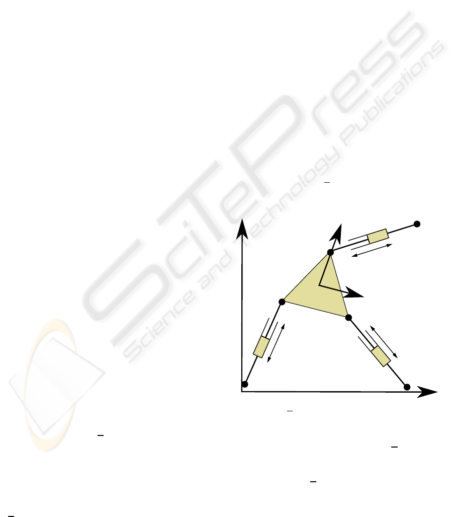
Figure 1 shows a 3-RP
R robot, which has three
joints in each serial link. R stands for a rotatory joint
and P stands for a prismatic joint whereby the under-
line signifies the joint which is actuated (Siciliano and
Khatib, 2007).
The forward kinematics function of a parallel has
been studied in detail in the literature, especially for a
3-RP
R robot. (Kong, 2008) derived algebraic expres-
B
1
B
2
B
3
A
1
A
2
A
3
Platform
Figure 1: A 3-RPR planar parallel manipulator. B
1
, B
2
, and
B
3
are connected to a stationary base.
sions for the forward kinematics of a 3-RPR robot and
analyzed its singularities. (Collins, 2002) used pla-
nar quaternions to formulate kinematic constraints in
equations for a 3-RPR robot. (Murray et al., 1997)
used coefficients of a constraint manifold, which are
functions of the locations of the base and platform
joints and the distance between them, for the kine-
280
Saad Saleem M., A. Sultan I. and A. Khan A. (2009).
ANALYTICAL KINEMATICS FRAMEWORK FOR THE CONTROL OF A PARALLEL MANIPULATOR - A Generalized Kinematics Framework for Parallel
Manipulators.
In Proceedings of the 6th International Conference on Informatics in Control, Automation and Robotics - Robotics and Automation, pages 280-286
DOI: 10.5220/0002214102800286
Copyright
c
 SciTePress

matics synthesis of a 3-RPR robot. (Wenger et al.,
2007) studied the degeneracy in the forward kinemat-
ics of a 3-RPR robot. (Kim et al., 2000; Dutre et al.,
1997) found the analytical Jacobian for a parallel ma-
nipulator. However, there is no attempt in literature
to formulate analytically the forward kinematics func-
tion for non-redundantparallel manipulators. The for-
ward kinematics function relates the joint variables of
the active joints to the position of the end-effector.
In the following section , the structure of the for-
ward and inversekinematics blocks is layed out. Then
forward kinematics function of a parallel manipulator
is derivedusing the position-closure property. The an-
alytical Jacobian of a parallel manipulator is also ob-
tained as described in the literature. Finally, a frame-
work to control a parallel manipulator is proposed,
followed by an example for the forward kinematics
function of a 3-RPR robot.
2 KINEMATICS FRAMEWORK
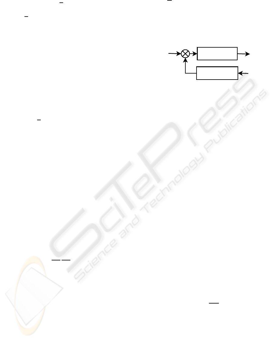
If the task is given in operational space then it be-
comes inevitable to cater for the non-linearities in-
troduced by the forward and inverse kinematics func-
tions. First, the joint variables are translated into op-
erational space. The resultant is compared to the ref-
erence trajectory and the error is then converted back
to joint space, as shown in Figure 2.
Suppose there are n serial manipulators in a paral-
lel manipulator that has n
a
active joints and n
p
pas-
sive joints such that the total number of joints is
n
c
= n
a
+ n
p
. If x is the end-effector position and F
is the forward kinematics function then the following
definitions can be introduced;
x = F (1)
˙x =
F
∂q
a
∂q
a
∂t
= J
c
˙q
a
(2)
¨x = J
c
¨q
a
+
˙
J
c
˙q
a
(3)
where ˙• signifies differentiation with respect to time,
J
c
is the systems Jacobian,
˙
J
c
is its time-derivate, and
q
a
is a vector of active joint variables. These variables
are in radians if the joint is revolute or in meters if the
joint is prismatic.
Equations (1), (2), and (3) can be combined as fol-
lows;


x
˙x
¨x


=


F
c
0 0
0 J
c
0
0
˙
J
c
J
c




q
a
˙q
a
¨q
a


(4)
or


x
˙x
¨x


= N
1
y (5)
where F
c
,
F
q
a
is the forward kinematics function that
relates the active joints to the end-effector position
and
N
1
,


F
c
0 0
0 J
c
0
0
˙
J
c
J
c


∈ ℜ
3n
c
×3l
(6)
-
Inverse kinematics
Forward kinematics
trajectory
Operational space
Joint
space
Figure 2: Operational space control of a parallel manipula-
tor.
The above matrix produces large values for small
values of q
a
. To avoid this situation, a limit is im-
posed here on the value of each component of q
a
so
that there is always a valid solution available.
The difference between the reference operational
space trajectory and the output of the forward kine-
matics block is referred to in this paper as system
error. Let

∆x,∆˙x, ∆ ¨x

T
be this error in operational
space. If this error is small, then (2) can be approxi-
mated to
∆x ≈ J
c
∆q
a
(7)
However, it can be stated, without any approxima-
tion, that
∆˙x = J
c
∆ ˙q
a
(8)
Ƭx =
˙
J
c
∆ ˙q
a
+ J
c
∆ ¨q
a
(9)
It is a common practice that when end-effector tra-
jectory is formulated in operational space, ∆x is cho-
sen in (7) such that the approximate movement of the
end-effector partially matches the target velocities in
(8) (Whitney, 1969). Equation (7) is only valid for a
small value of ∆x. If the target position is too distant,
it is important to bring the target closer. This way, the
manipulator reaches its final target in smaller steps.
For this reason, ∆x needs to be clamped such that
clamp(∆x,D
max
) =
(
∆x if ||∆x|| < D
max
D
max
∆x
||∆x||
otherwise
(10)
where || • || is the Euclidean norm. The value of the
scalar D
max
should be at least several times larger than
what end-effector moves in a single step and less than
half the length of a typical link. This heuristic ap-
proach has also been reported to reduce oscillations in
the system, which allows the designer to use a smaller
value for damping constant. This usually results in a
quicker response (Buss and Kim, 2005). To calculate
the error in joint space, (7), (8), and (9) can be written
ANALYTICAL KINEMATICS FRAMEWORK FOR THE CONTROL OF A PARALLEL MANIPULATOR - A
Generalized Kinematics Framework for Parallel Manipulators
281

as
∆q
a
= J
†
c
∆x (11)
∆ ˙q
a
= J
†
c
∆˙x (12)
∆ ¨q
a
= J
†
c
(∆¨x−
˙
J
c
∆ ˙q
a
)
= J
†
c
∆¨x − J
†
c
˙
J
c
J
†
c
∆˙x (13)
In matrix form, these equations can be written as


∆q
a
∆ ˙q
a
∆ ¨q
a


=


J
†
c
0 0
0 J
†
c
0
0 −J
†
c
˙
J
c
J
†
c
J
†
c




∆x
∆˙x
Ƭx


(14)
or alternatively
∆y = N
2


∆x
∆˙x
Ƭx


(15)
where J
†
c
is the pseudoinverse of J
c
. Pseudoinverse is
defined for all matrices including the ones which are
not square or are not full rank. It also gives the best
solution in terms of least squares. Except near sin-
gularities, the pseudoinverse gives a stable solution
even in those cases when the target end-effector posi-
tion doesn’t lie in the work volume of the mechanical
manipulator. The resulting solution is the closest lo-
cation to its target which minimizes ||J
c
∆q− ∆x||
2
. In
the vicinity of singularity, the pseudoinverse creates
large changes in joint variables, even for very small
changes in the end-effector position, resulting in an
unstable system. One important feature of pseudoin-
verse is that the term (I − J
†
c
J
c
) projects on the null
space of J
c
. This feature can be exploited for redun-
dant manipulators. It is possible to generate internal
motions in a redundant manipulator, i.e., ˙q
0
, without
changing its end-effector position (Sciavicco and Si-
ciliano, 2000). For redundant manipulators, (2) can
be written as
˙x = J
c
˙q+ (I − J
†
c
J
c
) ˙q
0
(16)
However, in this paper it is assumed that the paral-
lel manipulator is not redundant, i.e., number of active
joints is equal to the DOF of the end-effector.
The damped least-squares (DLS) method, which
is also referred to the Levenberg-Marquardt method,
solves many problems related to pseudoinverse. The
method gives a numerically stable solution near sin-
gularities, and was first used in inverse kinematics
by (Wampler, 1986) and (Nakamura and Hanafusa,
1986). It was also used for theodolite calibration by
(Sultan and Wager, 2002).
Not only does DLS minimize the term ||J
c
˙q
a
− ˙x||
2
but it also minimizes the joint velocities with a damp-
ing factor, i.e., λ
2
|| ˙q
a
||
2
where λ ∈ ℜ and λ 6= 0. The
function to be minimized can be written as
min
˙q
a
n
||J
c
˙q
a
− ˙x||
2
+ λ
2
|| ˙q
a
||
2
o
(17)
The DLS solution is equal to (Buss and Kim,
2005)
˙q
a
= (J
T
c
J
c
+ λ
2
I)
−1
J
T
c
˙x (18)
or alternatively
˙q
c
= J
T
c
(J
c
J
T
c
+ λ
2
I)
−1
˙x (19)
Equation (18) requiresan inversionof an n×n ma-
trix, while (19) requires an inversion of only an l × l
matrix, which is computationally more efficient. In
terms of SVD, the singular values change from
1
σ
i
for
J
†
c
to
σ
2
σ
2
+λ
2
for (J
c
J
T
c
+ λ
2
I)
−1
(Buss and Kim, 2005).
If σ
i
 0,
1
σ
i
 ∞, while in the other case,
σ
2
σ
2
+λ
2

1
λ
2
when σ
i
 0. Therefore, a stable solution is observed
even near singularities for ∀λ : λ 6= 0. Using (19), N
2
can be redefined as
N
2
,


J
∗
c
0 0
0 J
∗
c
0
0 −J
∗
c
˙
J
c
J
∗
c
J
∗
c


∈ ℜ
3l×3n
c
(20)
where J
∗
c
= J
T
c
(J
c
J
T
c
+ λ
2
I)
−1
. The value of λ is set
by the designer. Large values can result in a slower
convergence rate and very small values can reduce
the effectiveness of the method. In literature, there
are many methods proposed to select the value of λ
dynamically (Mayorga et al., 1990; Nakamura and
Hanafusa, 1986; Chiaverini et al., 1994).
3 FORWARD KINEMATICS
FUNCTION
In order to formulate the forward and inverse kine-
matics matrices, N
1
and N
2
, it is important to formu-
late analytically the forward kinematics function of
a parallel manipulator. The derivation is somewhat
similar to the derivation of the analytic Jacobian of
a parallel manipulator by (Dutre et al., 1997), which
was derived using the velocity-closure property. The
derivation is given as follows;
As all the manipulators are connected to the same
end-effector, it can be stated, using the position-
closure property, that
F
c
q
a
= F
1
q
1
= F
2
q
2
= ··· = F
n
q
n
(21)
where q
j
is the vector of joint variables of j
th
ma-
nipulator and F
j
(q) ,
F
j
(q)
q
j
is the forward kinematics
function of the j
th
manipulator.
Each column of the function F
c
corresponds to ro-
tational angle or displacement of an active joint, de-
pending on whether the joint is rotatory or prismatic.
Hence
F
i
c
= F
j
q
i
j
(22)
ICINCO 2009 - 6th International Conference on Informatics in Control, Automation and Robotics
282

where F
i
c
∈ ℜ
n
a
is the i
th
column of F
c
and q
i
j
is a
vector of joint variables of the j
th
manipulator when
the i
th
active joint is movedone unit while all the other
active joints are locked. If q
c
is the vector of all the
joint variables, i.e.,
q
c
=




q
1
q
2
.
.
.
q
n
c




∈ ℜ
n
c
(23)
then (22) can be written as
F
i
c
= F
j
S
j
q
i
c
(24)
where q
i
c
is a vector of all the joints when the i
th
active
joint is moved one unit while all the other active joints
are locked and S
j
is a selection matrix to select the
variables of the j
th
manipulator, i.e.,
S
j
=




0 ... 1 0 ... 0 ... 0
0 ... 0 1 ... 0 ... 0
.
.
.
.
.
.
.
.
.
.
.
.
.
.
.
.
.
.
.
.
.
.
.
.
0 ... 0 0 ... 1 ... 0




∈ ℜ
n
j
×n
c
where n
j
is the number of joints in the j
th
manipula-
tor. Let q
p
be the vector of passive joint variables and
q
a
be the vector of active joint variables such that
q
p
= S
p
q
c
(25)
q
a
= S
a
q
c
(26)
where q
p
∈ ℜ
n
p
and q
a
∈ ℜ
n
a
and S
p
and S
a
are se-
lection matrices for passive and active joints, respec-
tively. Typical values of S
p
and S
a
can be written as
S
p
=



... 0 1 0 ... 0 0 0 .. .
.
.
.
.
.
.
.
.
.
.
.
.
.
.
.
.
.
.
.
.
.
.
.
.
.
.
.
... 0 0 0 ... 0 1 0 .. .



∈ ℜ
n
p
×n
c
and
S
a
=



... 0 0 0 ... 0 1 0 ...
.
.
.
.
.
.
.
.
.
.
.
.
.
.
.
.
.
.
.
.
.
.
.
.
.
.
.
... 0 1 0 ... 0 0 0 ...



∈ ℜ
n
a
×n
c
Both of these matrices are sparse and orthogonal,
i.e., S
p
S
T
p
= I and S
a
S
T
a
= I, which implies
q
c
p
= S
T
p
q
p
(27)
q
c
a
= S
T
a
q
a
(28)
where q
c
p
is equivalent to q
c
except that the active
joints are set to zero and similarly, q
c
a
is equivalent to
q
c
except that the passive joints are set to zero such
that
q
c
= q
c
p
+ q
c
a
(29)
Substituting (27) and (28) in (29) yields
q
c
= S
T
p
q
p
+ S
T
a
q
a
(30)
In reference to the position-closure property (21),
let
Aq
c
= 0 (31)
where
A =






F
1
q
1
−
F
2
q
2
0 ... 0
F
1
q
1
0 −
F
3
q
3
... 0
.
.
.
.
.
.
.
.
.
.
.
.
.
.
.
F
1
q
1
0 0 ... −
F
n
q
n






∈ ℜ
n
a
(n−1)×n
c
(32)
Substituting the value of q
c
from (30) gives
Aq
c
= A(q
c
p
+ q
c
a
)
= AS
T
p
q
p
+ AS
T
a
q
a
= A
p
q
p
+ A
a
q
a
(33)
Applying (31)
q
p
= −A
†
p
A
a
q
a
(34)
Substituting this expression in (30) yields
q
c
= S
T
a
q
a
− S
T
p
A
†
p
A
a
q
a
(35)
As q
i
c
is defined for a unit displacement of the i
th
active joint, hence, q
a
can be replaced with a column
of S
a
which corresponds to the i
th
active joint, denoted
by (S
a
)
i
, to evaluate q
i
c
, i.e.,
q
i
c
= S
T
a
(S
a
)
i
− S
T
p
A
†
p
A
a
(S
a
)
i
(36)
Substituting the above value in (24) gives
F
i
c
= F
j
S
j
q
i
c
(37)
or
F
c
= F
j
S
j

q
1
c
q
2
c
... q
n
a
c

(38)
4 ANALYTICAL JACOBIAN AND
ITS DERIVATIVE
(Dutre et al., 1997) evaluated the analytical Jacobian
for a parallel manipulator using the velocity-closure
property. The Jacobian can also be derived by replac-
ing F
c
in (38) by J
c
and q
i
c
by ˙q
i
c
, i.e.,
J
c
= J
j
S
j

˙q
1
c
˙q
2
c
... ˙q
n
a
c

(39)
where J
c
is the analytical Jacobian that relates the ve-
locities of the active joints to the end-effector velocity.
J
j
and ˙q
j
are the Jacobian and the vector of joint ve-
locities of the j
th
manipulator, respectively. ˙q
i
c
can be
stated using (36) as follows;
˙q
i
c
= S
T
a
(S
a
)
i
− S
T
p
B
†
p
B
a
(S
a
)
i
(40)
ANALYTICAL KINEMATICS FRAMEWORK FOR THE CONTROL OF A PARALLEL MANIPULATOR - A
Generalized Kinematics Framework for Parallel Manipulators
283

where B
p
= BS
T
p
, B
a
= BS
T
a
, and
B =




J
1
−J
2
0 ... 0
J
1
0 −J
3
... 0
.
.
.
.
.
.
.
.
.
.
.
.
.
.
.
J
1
0 0 0 −J
n




∈ ℜ
n
a
(n−1)×n
c
(41)
Using B, the velocity-closure propertyof a parallel
manipulator can be written as
B˙q
c
= 0
The derivative of the closed-loop Jacobian (J
c
)
given in (39) is
˙
J
c
=
˙
J
j
S
j

¨q
1
c
¨q
2
c
... ¨q
n
a
c

(42)
where ¨q
i
c
can be calculated by differentiating (40), i.e.,
¨q
i
c
= −S
T
p
∂B
†
p
∂q
i
B
a
+ B
†
p
∂B
a
∂q
i
!
(S
a
)
i
(43)
where q
i
is the i
th
driving joint.
The time derivative of a Jacobian column for a se-
rial manipulator is the sum of the partial derivatives of
this column with respect to joint variables, multiplied
by the time-derivates of these variables (Bruyninckx
and De Schutter, 1996). As such, time-derivative of
the i
th
column of the Jacobian is given by
˙
J
i
=
n
∑
j=1
∂J
i
(q)
∂q
j
∂q
j
∂t
=
n
∑
j=1
∂J
i
(q)
∂q
j
˙q
j
(44)
Similarly, the derivative of the Jacobian of each
manipulator of a parallel manipulator can be ex-
pressed using (44), i.e.,
˙
J
j
=
n
a
∑
i=1
∂J
j
∂q
i
˙q
i
=
n
a
∑
i=1
n
j
∑
k=1
∂J
j
∂q
j,k
∂q
j,k
∂q
i
!
˙q
i
(45)
where k is a joint of the j
th
manipulator and
∂J
j
∂q
j,k
rep-
resents Jacobian derivative of the j
th
serial manipula-
tor. The factor,
∂q
j,k
∂q
i
in (45), is the k
th
component in
S
j
˙q
i
c
.
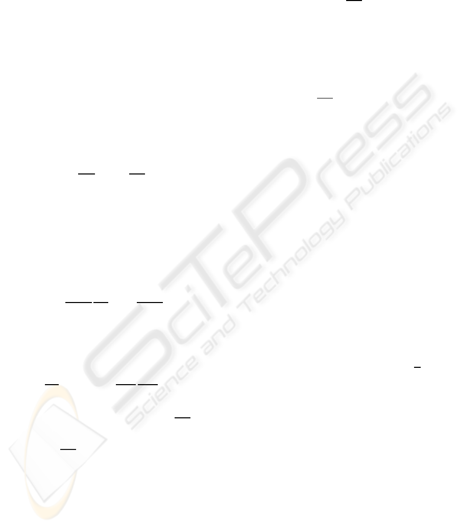
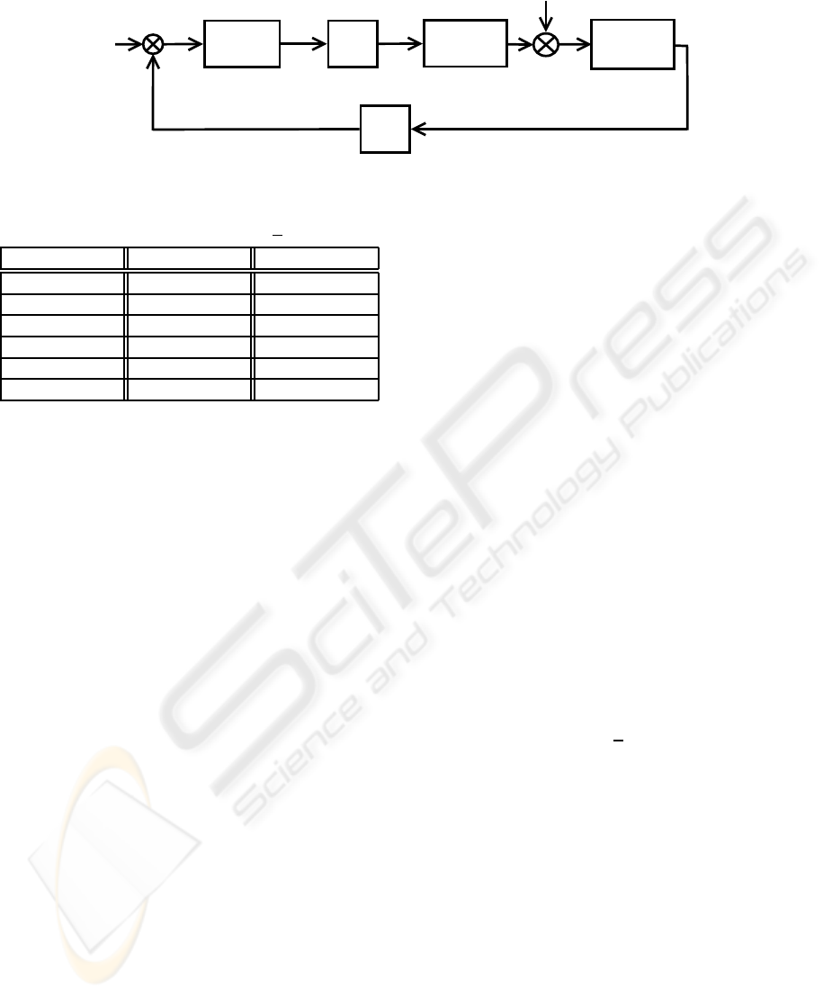
5 PROPOSED CONTROL
FRAMEWORK
Figure 3 shows the structure of the proposed con-
trol framework for parallel manipulators. As only ac-
tive joints are actuated, it is important to incorporate
the contribution of the passive joints onto the active
joints. If joint friction is ignored, the relationship be-
tween the torque of active joints and passive joints is
given by the following equation (Cheng et al., 2003);
τ
c
= τ
a
+

∂q
p
∂q
a

T
τ
p
(46)
where τ
p
∈ ℜ
n
p
is the torque measured from strain
gauges on passive joints, τ
a
∈ ℜ
n
a
is the torque pro-
duced by the actuators on active joints, and τ
c
∈ ℜ
n
a
is the torque measured by strain gauges mounted on
active joints. From (Dutre et al., 1997), it can be in-
ferred that
∂q
p
∂q
a
= B
†
p
B
a
Using the above value in (46) yields
τ
c
= τ
a
− (B
†
p
B
a
)
T
τ
p
or
τ
c
= τ
a
− B
T
a
(B
†
p
)
T
τ
p
(47)
The passive joints project torque onto the active
joints with a factor of −B
T
a
(B
†
p
)
T
. This will be used as
the exogenous force disturbance signal in the hybrid
controller, as shown in Figure 3.
To ease the implementation of the clamp block, it
can be taken out of the closed loop. This can be done
by redefining r
k
using
r
k
= clamp(r
original
− N
1
y
k
) + N
1
y
k
(48)
6 EXAMPLE
As the proposed kinematics framework is evaluated
analytically, it can be applied on any non-redundant
parallel manipulator. However, in this section, for the
sake of demonstration, a simple case of a 3-RPR robot
is presented, shown in Figure 1.
The forward kinematics function for the first ma-
nipulator can be stated as
F
1
=


(x
1,1
+ q
1,2
+ x
1,2
)cos(q
1,1
) + x
1,3
cos(q
1,1
+ q
1,3
)
(x
1,1
+ q
1,2
+ x
1,2
)sin(q
1,1
) + x
1,3
sin(q
1,1
+ q
1,3
)
q
1,1
+ q
1,3


(49)
where x
1,2
and q
1,2
denote the length of the second
link and the second joint variable, respectively. The
expressions for other links can be written in the same
way. Using this kinematic model for the values given
in Table 1, the end-effector position was found to be
at
x
end
c
=


1.5
2.5981
1.0472


where the first two elements represent the position in
x− y plane and the third element represents the angu-
lar rotation of the end-effector.
ICINCO 2009 - 6th International Conference on Informatics in Control, Automation and Robotics
284

-
clamp


∆x
∆˙x
Ƭx


N
2
N
1
Controller
Manipulator


∆q
∆ ˙q
∆ ¨q


τ
a
τ
c
−B
T
a
(B
†
p
)
T
τ
p
y =


q
˙q
¨q


r
k
=


x
r
˙x
r
¨x
r


Figure 3: Operational space control of a parallel manipulator.
Table 1: Assumed values for a 3-RPR robot.
Manipulator 1 Manipulator 2 Manipulator 3
q
1,1
= π/3 q
2,1
= 2π/3 q
3,1
= 4π/3
q
1,2
= 1 q
2,2
= 1 q
3,2
= 1
q
1,3
= 0 q
2,3
= −π/3 q
3,3
= −π
x
1,1
= 0.5 x
2,1
= 0.5 x
3,1
= 0.5
x
1,2
= 0.5 x
2,2
= 0.5 x
3,2
= 0.5
x
1,3
= 1 x
2,3
= 1 x
3,3
= 1
The forward kinematics function, F
c
, gives the
following end-effector position for the active joints

1,1,1

T
;
x
end
=


1.498
2.597
1.048


7 CONCLUSIONS
Similar to the analytical Jacobian for a parallel ma-
nipulator, which is a function of joint variables and
relates the velocity of the active joints to the velocity
of the end-effector, the analytical forward kinematics
function is also a function of the joint variables that
relates the position of the active joints to the position
of the end-effector. The generality of the proposed
technique allows the forward kinematics function to
be used in a variety of applications. A control config-
uration is also described in this paper as a prospective
application of the proposed technique.
REFERENCES
Bhattacharya, S., Hatwal, H., and Ghosh, A. (1997). An
on-line parameter estimation scheme for generalized
Stewart platform type parallel manipulators. Mecha-
nism and Machine Theory, 32(1):79–89.
Bruyninckx, H. and De Schutter, J. (1996). Symbolic
differentiation of the velocity mapping for a serial
kinematic chain. Mechanism and Machine Theory,
31(2):135–148.
Buss, S. and Kim, J. (2005). Selectively Damped Least
Squares for Inverse Kinematics. Journal of Graphics
Tools, 10(3):37–49.
Cheng, H., Yiu, Y.-K., and Li, Z. (2003). Dynamics
and control of redundantly actuated parallel manip-
ulators. IEEE/ASME Transactions on Mechatronics,
8(4):483–491.
Chiaverini, S., Siciliano, B., and Egeland, O. (1994). Re-
view of the damped least-squares inverse kinematics
with experiments on an industrial robot manipulator.
IEEE Transactions on Control Systems Technology,
2(2):123–134.
Collins, C. (2002). Forward kinematics of planar parallel
manipulators in the Cliffordalgebra of P2. Mechanism
and Machine Theory, 37(8):799–813.
Dutre, S., Bruyninckx, H., and De Schutter, J. (1997).
The analytical jacobian and its derivative for a par-
allel manipulator. In IEEE International Conference
on Robotics and Automation, volume 4, pages 2961–
2966.
Kim, D., Chung, W., and Youm, Y. (2000). Analytic ja-
cobian of in-parallel manipulators. In Proceedings of
the IEEE International Conference on Robotics and
Automation ICRA ’00, volume 3, pages 2376–2381.
Kong, X. (2008). Advances in Robot Kinematics: Analysis
and Design, chapter Forward Kinematics and Singu-
larity Analysis of a 3-RPR Planar Parallel Manipula-
tor, pages 29–38. Springer Netherlands.
Mayorga, R., Milano, N., and Wong, A. (1990). A simple
bound for the appropriate pseudoinverse perturbation
of robot manipulators. In Proceedings of the IEEE In-
ternational Conference on Robotics and Automation,
volume 2, pages 1485–1488.
Murray, A., Pierrot, F., Dauchez, P., and McCarthy, J.
(1997). A planar quaternion approach to the kine-
matic synthesis of a parallel manipulator. Robotica,
15(04):361–365.
Nakamura, Y. and Hanafusa, H. (1986). Inverse kinematic
solutions with singularity robustness for robot manip-
ulator control. Journal of dynamic systems, measure-
ment, and control, 108(3):163–171.
Sciavicco, L. and Siciliano, B. (2000). Modelling and Con-
trol of Robot Manipulators. Springer, second edition.
Siciliano, B. and Khatib, O. (2007). Springer Handbook of
Robotics. Springer-Verlag, Secaucus, NJ, USA.
ANALYTICAL KINEMATICS FRAMEWORK FOR THE CONTROL OF A PARALLEL MANIPULATOR - A
Generalized Kinematics Framework for Parallel Manipulators
285

Sultan, I. and Wager, J. (2002). Simplified theodolite cal-
ibration for robot metrology. Advanced Robotics,
16(7):653–671.
Timmons, K. and Ringelberg, J. (2008). Approach and Cap-
ture for Autonomous Rendezvous and Docking. In
2008 IEEE Aerospace Conference, pages 1–6.
Wampler, C. W. (1986). Manipulator inverse kinematic
solutions based on vector formulations and damped
least-squares methods. IEEE Transactions on Sys-
tems, Man, and Cybernetics, 16(1):93–101.
Warnecke, H., Neugebauer, R., and Wieland, F. (1998). De-
velopment of Hexapod Based Machine Tool. CIRP
Annals-Manufacturing Technology, 47(1):337–340.
Wenger, P., Chablat, D., and Zein, M. (2007). Degener-
acy Study of the Forward Kinematics of Planar 3-RPR
Parallel Manipulators. Journal of Mechanical Design,
129:1265.
Whitney, D. E. (1969). Resolved motion rate control of ma-
nipulators and human prostheses. IEEE Transactions
on Man Machine Systems, 10(2):47–53.
Yamane, K., Nakamura, Y., Okada, M., Komine, N., and
Yoshimoto, K. (2005). Parallel Dynamics Computa-
tion and H
∞
Acceleration Control of Parallel Manip-
ulators for Acceleration Display. Journal of Dynamic
Systems, Measurement, and Control, 127:185.
ICINCO 2009 - 6th International Conference on Informatics in Control, Automation and Robotics
286